Plane-Stress/Plate Stresses
Check the stress distribution of plane-stress elements or plate elements in Contours.
From the Main Menu select Results > Results > Stresses > Plane-Stress/Plate Stresses.
 Load Cases/Combinations
Select a desired load case, load combination or envelope case.
Click
![]() to the right to enter new or modify existing load combinations.
(Refer to "Load
Cases / Combinations")
to the right to enter new or modify existing load combinations.
(Refer to "Load
Cases / Combinations")
Step
Specify the step for which the analysis results are to be produced.
The Step is defined in geometric nonlinear analysis as Load Step,
and additional steps are defined in the construction stages of
heat of hydration analysis etc.
Note 1
The Construction Stage applicable for the output of the construction
stage analysis is defined in Select
Construction Stage for Display or Stage Toolbar.
Note 2
When pushover analysis is performed for a structure containing Plate, Plane Stress or Solid elements, the pushover analysis results for Plate, Plane Stress or Solid elements can be produced by Steps.
|
Components
Select the desired stress component among the following:
For UCS
Sig-XX: Axial stress in GCS X-direction
Sig-YY: Axial stress in GCS Y-direction
Sig-ZZ: Axial stress in GCS Z-direction
Sig-XY: Shear stress in GCS X-Y plane
Sig-YZ: Shear stress in GCS Y-Z plane
Sig-XZ: Shear stress in GCS X-Z plane
Sig-Max: Maximum Principal Stress
Sig-Min: Minimum Principal Stress
Sig-EFF: Effective stress (von-Mises Stress)
Max-Shear: Maximum shear stress (Tresca Stress)
For Local
Sig - xx: Axial stress in the element's local x-direction (Perpendicular to local y-z plane)
Sig - yy: Axial stress in the element's local y-direction (Perpendicular to local x-z plane)
Sig - xy: Shear stress in the element's local x - y plane (In-plane shear stress)
Vector: Display the maximum and minimum principal stresses in vectors
Vector Scale Factor: Drawing scale for the vector diagram
Type of Display
Define the type of display as follows :
Contour |
Display the stresses of plane-stress/plate elements in contour.
|
|
Ranges: Define the contour ranges.
Number of Colors: Assign
the number of colors to be included in the contour (select
among 6, 12, 18, 24 colors) Colors: Assign or control the colors of the contour. Color Table: Assign the type of Colors.
Reverse Contour: Check on to reverse the sequence of color variation in the contour. Contour Line: Assign the boundary line color of the contour Element Edge: Assign
the color of element edges while displaying the contour Contour Options: Specify options for contour representation Contour Fill Gradient Fill: Display
color gradient (shading) in the contour. Draw Contour Line Only Mono line: Display the boundaries of the contour in a mono color. Contour Annotation Spacing: Specify the spacing of the legend or annotation. Coarse Contour (faster)
(for large plate or solid model) Extrude
|
Deform |
Display the deformed shape of the model.
|
|
Deformation Scale Factor Deformation Nodal Deform: Display
the deformed shape reflecting only the nodal displacements. Real Displacement (Auto-Scale
off): The true deformation of the structure is
graphically represented without magnifying or reducing
it. This option is typically used for geometric nonlinear
analysis reflecting large displacement. Relative Displacement: The deformation of the structure is graphically represented relative to the minimum nodal displacement, which is set to "0"
|
Values |
Display the
stresses of plain-stress/plate elements in numerical values. |
|
Decimal Points: Assign
decimal points for the displayed numbers Min & Max: Display
the maximum and minimum values Set Orientation: Display orientation of numerical values Note
|
Legend |
Display various references related to analysis results to the right or left of the working window.
|
|
Legend Position: Position of the legend in the display window Rank
Value Type: Specify a type of values in the Legend
and the number of decimal points. |
Animate |
Dynamically
simulate the stresses of the plain-stress/plate elements.
|
|
Animation Mode: Determine the type of animation for analysis results. Animate Contour: Option
to change the color of the contour representing the transition
according to the magnitudes of variation Note AVI Options: Enter the options required to produce the animation window. Bits per Pixel: Number
of bits per pixel to create the default window for animation Construction Stage Option: Select the animation options when the construction stage analysis is performed. Stage
Animation: Animations by construction stages |
Undeformed |
Overlap the undeformed and deformed shapes of the model.
|
Mirrored |
"Mirrored" allows the user to expand the analysis results obtained from a half or quarter model into the results for the full model by reflecting planes.
|
|
Half
Model Mirroring |
Disp. Opt. |
Plate stress contour can be displayed using the value at the element center instead of element node. Plate stresses at the nodes are determined by the linear interpolation of Gauss points, which often leads to stress exceeding yield stress. The center values will rarely exceed the yield stress. |
|
|
Yield Point |
If the analysis results produced by material nonlinear analysis exceed the yield stress of Plastic Material defined in Initial Uniaxial Yield Stress, Hinge is produced at Gauss Point. |
|
|
Note 1
Yield Point is applicable in Plane Stress Elements and Plate Elements.
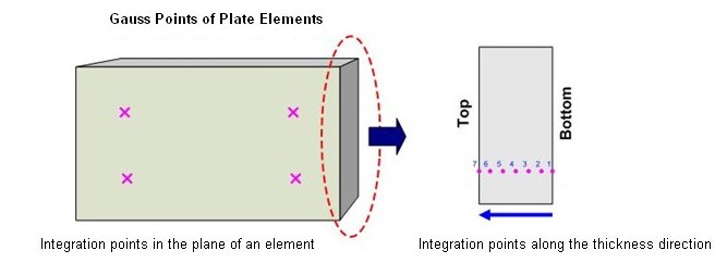
Note 2
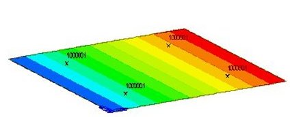
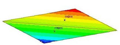
For displaying Yield Points on a Plate Element, a Laminated Shell model with 7 layers has been used in order to consider material nonlinear analysis. To check the yield state of Gauss Points, "0,1" is applied from bottom to top. "0" represents the state of elasticity and "1" the state of yielding. For rectangular or triangular elements, the method of displaying "0,1" is identical.
|
|
Rectangular Element |
Triangular Element |
Cutting Diagram |
Graphically
display the stresses of the plain-stress/plate elements
along the cutting line or plane. |
|
Click
|
Plate Cutting Diagram Mode
Cutting Line: Produce a graph along a cutting line
Cutting Plane: Produce a graph along the line of intersection of the cutting plane and plate elements
![]() When
Cutting Plane is selected
When
Cutting Plane is selected
 Batch Output Generation (
.jpg) ,
, .jpg) )
)
Given the types of analysis results for Graphic outputs, generate consecutively graphic outputs for selected load cases and combinations. A total number of files equal to the products of the numbers of checked items in the three columns of the dialog box below are created.
|
Assign
a Base File Name under which the types of results (selection
data in the Batch Output Generation dialog box for graphic
outputs) are stored. |
|
Specify the Base Files to perform Batch Output Generation, construction stages, load cases (combinations), steps, etc. in the following dialog box. |
Saved Menu-Bar Info's: Listed here are the Base Files. Select the Base File Names for Batch Output.
![]() : Delete all the
Base Files selected with the mouse.
: Delete all the
Base Files selected with the mouse.
When the construction stage analysis is carried out, all the construction stages are listed. We simply select the stages of interests to be included in the batch output. If no construction stage analysis is performed, the column in the dialog box becomes inactive and lists load (combination) conditions.
Stages
The results output of all the construction stages are produced.
The construction stages are listed below.
Final
Stage Loads
The results output for only the Final Stage are produced. The construction
stages are listed below. If no construction stage analysis is
performed, the load (combination) conditions are listed.
Use
Saved
Apply only the (saved) step or load (combination) condition selected
at the time of creating each Base File.
Stage
LCase/LComb
When the construction stage analysis is carried out, the auto-generated
construction stage load conditions and the additionally entered
construction stage load combinations are listed. Check on only
the load (combination) conditions that will be used to produce
batch outputs. This column becomes inactive if "Final Stage
Loads" is selected or no construction stage analysis is carried
out.
Step
Option
Specify the steps for which the outputs will be produced when the
construction stage analysis or large displacement geometric nonlinear
analysis is performed.
Saved Step: Use only the steps used for creating the Base Files
All Steps: Use all the steps
Output Options
Output
File Type
Select a Graphic File type, either BMP or EMF.
Auto
Description: At the top left
of the Graphic Outputs produced in batch, auto-generate and include
the notes such as the types and components of the analysis results,
construction stages and steps, load (combination) conditions,
etc. The font size, color, type, etc. can be changed upon clicking
the button ![]() .
.
Output
Path
Specify the path for saving the graphic files to be produced in
batch.
File Prefix: Specify the prefix of the Graphic Files to be created. The filenames will be consisted of "Prefix"_"Base File Name"_"Load Comb.".bmp(emf) or "Prefix"_"Base File Name"_"Stage"_"Stage LCase"_"Step".bmp(emf).
![]() : Produce
the specified batch Graphic Files reflecting the contents of the
dialog box.
: Produce
the specified batch Graphic Files reflecting the contents of the
dialog box.
![]() /
/ ![]()
Produce the contents of data
input in the Base Files and Batch Output Generation dialog box
in a binary type file (fn.bog). Click the ![]() button and select a fn.bog to use the same output format.
button and select a fn.bog to use the same output format.
Note
Import /Export is only meaningful for different projects. In a
given structural model, the Base Files are automatically stored
and listed.