Define
the Construction Stage Set and then define the
Construction Stage.
A single file can be composed
of multiple Construction stage sets.
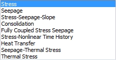
The construction stage
types are [Stress], [Seepage], [Stress-Seepage-Slope],
[Consolidation], [Fully Coupled stress], [Heat
Transfer], [Seepage-Thermal Stress], [Thermal
Stress].
Click the Define Construction
Stage button to form the construction stage. Advanced
options that are not available on the [Stage Definition
Wizard] can be set.
<Define
construction stage>
Stage
name
Define the construction
stage name. Use [New] to create a new construction
stage and use [Insert] to add a new construction
stage in between existing stages.
For example, clicking the
Insert button at Stage 2 moves the current stage
to Stage 3, and the new stage becomes Stage2.
Click the  button to move to
the previous or next stage. button to move to
the previous or next stage.
Stage
type
Specify the construction
stage type. Be aware that the designated [Analysis
Control], [Output Control] options are different
and the boundary conditions/loading conditions
for each stage type are different.
Refer to the Analysis >
Analysis case > General > Analysis/Output
Control for more information on control options.
Move
to Previous/Next
The construction stage
order may need modification when many construction
stages are created. Use the Move to Previous or
Next button to change the order of created construction
stages.
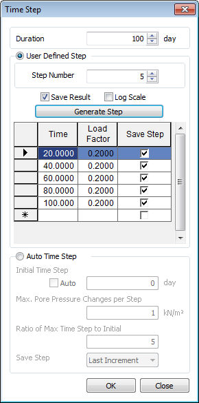
Time
Step
Define time steps used
in the analysis.
Insert
the duration to be analyzed. ‘User Defined Step’
generates steps by dividing with Step Number.
‘Auto Time Step’ automatically divides defined
period with time step.
It will
automatically choose appropriate time steps for
a seepage, consolidation, semi/fully coupled stress
seepage analysis and thermal analyses.
When the
calculation runs smoothly, resulting in very few
iterations per step, then the program will choose
a larger time step. When the calculation uses
many iterations due to an increasing amount of
plasticity, then the program will take smaller
time steps.
This function
reduces the pore water pressure result errors
when loading is applied in short period of time.
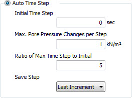 
Initial
Time Step can be either manually defined by user
or calculated automatically within solver. The
automatic calculation formula is as follows:
Input
Max. Pore Pressure Changes per step. When pore
pressure changes exceeds the maximum value, step
size is automatically reduced and analyzed.
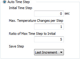
Input
Max. Temperature Changes per step. When temperature
changes exceeds the maximum value, step size is
automatically reduced and analyzed.
Input
the maximum value of time step ratio compared
to ‘Initial Critical Time Step’.
Select
the output method of results. 'Last Increment':
Only output results from last step, 'Every Increment':
Output results from all steps.
Set
Data
Display the usable Mesh
sets, Boundary sets, and Load sets in a worktree.
Be aware that the sub-sets are also displayed
independently, so take caution when selecting
the mesh sets.
For example, the set data
for the created Core mesh set with registered
mesh sub-sets (Core 001, Core 002, Core 003) are
shown in the right figure. In this case, activating
Core does not activate the mesh sub-sets Core
001, Core 002, Core 003. Hence, mesh sets that
are not registered directly on the set data are
useless.
Activated
Data
Register
the activated sets for each construction stage.
The activated sets remain active for future construction
stages without needing re-activation until it
is deactivated. The sets that need to be activated
for the construction stage can be selected using
the left mouse button and dragged & dropped
into the activated data. Another method is to
select the sets using the right mouse button on
the Set data and select activate on the Context
menu.
Deactivated
data
Register
the deactivated set for each construction stage.
The deactivated sets remain active for future
construction stages until they are re-activated.
The sets that need to be deactivated for the construction
stage can be selected using the left mouse button
and dragged & dropped into [Deactivated data].
Another method is to select the sets using the
right mouse button on [Set data] and select deactivate
on the Context menu.
Define
Water Level For Global
Input
the groundwater level that changes according to
the construction stage with respect to the GCS.
Click  to set the ground
water level function. If the water level and function
are both specified, the input water level is multiplied
onto the function and applied on the analysis. to set the ground
water level function. If the water level and function
are both specified, the input water level is multiplied
onto the function and applied on the analysis.
Define
Water Level for Mesh Set
Define
the groundwater level that changes according to
the construction stage for each mesh set.
If
the groundwater layer is surrounded by rocks or
an impermeable clay layer (confined aquifer),
the presence/absence of the groundwater level
for each ground layer can be set for analysis.
If
the total groundwater level is input and a mesh
set has a defined groundwater level, the mesh
set groundwater level has priority and the total
groundwater level is applied to mesh sets that
do not have a defined level.
If
the water level and function are both specified,
the input water level is multiplied onto the function
and applied on the analysis.
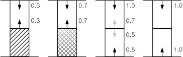
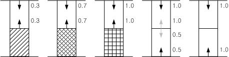
LDF
Set
the Load Distribution Factor. The sum of all distribution
factors need to be 1, and the keyboard Enter key
needs to be pressed after the input to apply the
value properly.
For the example case
shown below, a LDF of 0.4 is applied to the current
stage and a LDF of 0.3 is applied to the next
stage and the subsequent stage. Here, the LDF
does not need to be checked for the latter two
stages and the LDFs need to be set such that they
do not overlap in the construction stages.
|