Time History Load Cases
Define the conditions and required control data for time history analysis. The procedure for carrying out a time history analysis is outlined below.
1. Enter the mass data in the analysis model using the various mass input functions provided in the Model > Masses menu.
2. Recall the Analysis > Eigenvalue Analysis Control menu to enter various data required for eigenvalue analysis including the number of modes.
3. Select Load > Time History Analysis Data > Time
Forcing Functions and click ![]() to enter
the function name and related time forcing function.
to enter
the function name and related time forcing function.
4. Using Load > Time History Analysis Data > Time History Load Cases, enter the load case name, data related to the processes of time history analysis and output, and damping ratio.
5. If Time Forcing Function is entered as Dynamic Nodal Loads: Using Load > Time History Analysis Data > Dynamic Nodal Loads, select the Time History Load Case Name and Function Name for load application and enter the Loading Direction, Arrival Time, etc.
If Time Forcing Function is entered as ground motion: Using Load > Time History Analysis Data > Ground Acceleration, enter the Time History Load Case Name and directional Function Names, Angle of Horizontal Ground Acc., etc.
Time Forcing Function is entered as Time Varying Static Loads: Using Load > Time History Analysis Data > Time Varying Static Loads, select the Time History Load Case Name, Static Load and Function Name and enter the Loading Direction, Arrival Time, etc.
6. Select Analysis>Perform
Analysis or click ![]() Perform Analysis
to initiate the time history analysis.
Perform Analysis
to initiate the time history analysis.
7. When the analysis is successfully completed, we can then analyze the results and combine the results with static load cases using the various post-processing functions. All the analysis results are produced in maximum and minimum values that occurred during the time history. If the results in conjunction with varying time are of interest, we can produce time history output in graphs and texts using Results > Time History Results.
Time history analysis cannot be carried out along with the following analyses:
- Response Spectrum Analysis
- Buckling Analysis
- Large Displacement Analysis
- Material Nonlinear Analysis
- Heat of Hydration of Concrete
From the Main Menu select Load > Seismic > Time History Analysis Data > Time History Load Cases.
![]() To enter new or additional time
history analysis load cases
To enter new or additional time
history analysis load cases
Click ![]() .
.
![]() To modify previously entered
time history analysis load cases
To modify previously entered
time history analysis load cases
Select a load case from the time
history analysis load case list at the bottom of the dialog box,
then click ![]() and modify
the data entries.
and modify
the data entries.
![]() To delete previously entered
time history analysis load cases
To delete previously entered
time history analysis load cases
Select a load case from the time
history analysis load case list at the bottom of the dialog box
and click ![]() .
.
![]() :
Enter pertinent information for eigenvalue analysis.
:
Enter pertinent information for eigenvalue analysis.
 General
Name: Enter the name of the time history analysis load case. The name is used in "Combinations".
Description
State a brief description related to the time history load case
Analysis Type
Linear: Linear Time History Analysis
Nonlinear: Nonlinear Time History Analysis
Analysis Method
Modal: Modal Superposition Method
Direct Integration: Direct Integration Method
Static: Static Analysis. Pushover Analysis is possible by combining with Nonlinear from Analysis Type.
Note
Combination of Nonlinear Analysis and Static Analysis is equivalent to performing Pushover Analysis.
Time History Type
Transient: Time history analysis is carried out on the basis of loading a time load function only once. This is a common type for time history analysis of earthquake loads.
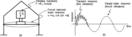
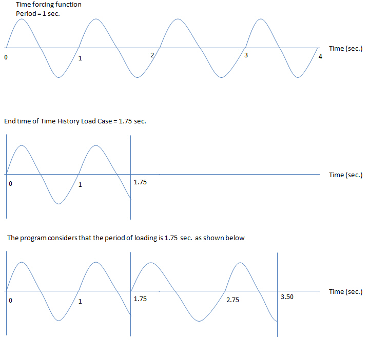
Periodic: Time history analysis on the basis of repeatedly loading a time load function, which has a period identical to End Time. This type is applicable for machine vibration loads.
Geometric Nonlinearity
Type
Select Large Displacement to consider the geometric nonlinear effect due to large displacement in Time History Analysis. This option is valid only when Analysis Type is "Nonlinear" and Analysis Method is "Direct Integration" or "Static".
End of Time
The finish time until which the time history analysis is required [Second]
Note
If the Time History Type is Transient, the analysis will be performed until the specified End Time. If the Time History Type is Periodic, the analysis will be repeated on the basis of the period identical to the End Time.
Time Increment
The time increment of a time history analysis significantly affects the accuracy of the analysis results. A common rule of thumb for determining the time increment is to use at least 1/10 of the smaller of the period of the time forcing function or the natural frequency of the structure. [Second]
Incremental Step
(Activates
only for the Nonlinear Static Analysis)
Enter the incremental steps until which the load will be incrementally applied to the structure. For example, if the number of incremental steps and the total load are 100 and 100 ton respectively in nonlinear static analysis, the load increases by 1 ton, and analysis is carried out for each step.
Step Number Increment
for Output
Analysis time step required for producing results of the time history analysis
Results produced at the interval of (Number of Output Steps x Time Increment)
Order in Sequential
Loading
Data related to a sequence of consecutively loaded multiple time history analysis conditions are entered here.
Subsequent to
Select a time history analysis condition previously defined, which precedes the time history analysis condition currently being defined. The Analysis Type and Analysis Method for the current time history analysis condition must be consistent with those for the preceding load condition. From the preceding analysis condition, displacement, velocity, acceleration, member forces, variables for the state of hinges and variables for the state of nonlinear link elements are obtained and used as the initial condition for analysis. However, in the case of loadings, the loading at the final state of the preceding analysis condition is assumed to constantly remain in the current analysis condition only when "Keep Final Step Constantly" is checked on.
Load Case: Select a preceding load case. In addition to the time history load (TH), the static load (ST) and the construction stage load (CS) can be also considered. It is not necessary to change a static load such as self weight to a time history load. A static load case can be directly selected.
Initial Element Forces (Table): It considers the equilibrium element forces due do the preceding load case. If a preceding load is applied from Load Case, it is limited to a load in the same structural system.
However, using Initial Element Forces (Table), it is possible to apply a preceding load to a structure whose boundary conditions change such as in earthquake analysis. The preceding load case can be in the form of equilibrium forces.
Initial Forces for Geometric Stiffness: Apply a preceding load to a structure using Initial Forces for Geometric Stiffness. It is valid when "Large Displacements" option is selected in Geometric Nonlinearity Type.
Note
This function considers Initial Element Forces entered in Loads>Initial Forces>Small Displacement>Initial Element Force Table as the preceding load case.
The preceding load case of static load, construction stage load, and equilibrium element forces do not support the fiber element. It is recommended that the member forces due to the preceding load case be kept in the elastic range. It may result in an inappropriate outcome beyond the elastic range.
Cumulative D/V/A Result: The displacement, velocity and acceleration results of a preceding load case are produced cumulatively. This does not affect the analysis itself. It is only applicable for a time history analysis load (TH).
Keep Final Step Loads Constant: The final step loads of the preceding load case are maintained. It is only applicable for a time history analysis load (TH).
Damping
Mass and Stiffness Proportional
Element Mass & Stiffness Proportional
Note
Significant unbalanced equilibrium forces may result in Direct
Modal and Strain Energy Proportional due to the damping characteristics.
As such, it is recommended to go through convergence calculation
if Direct Modal and Strain Energy Proportional are selected.
Static Loading Control
[Active only
for Nonlinear Static Analysis]
The program provides two control methods. Load Control Method increases loads by steps until the final load is reached and analyzes each step. Displacement Control Method increases displacements by steps until the target displacement is reached and analyzes each step.
Load Control
Scale Factor: Scale factor for loads used in Nonlinear Static Analysis
Displacement Control
Global Control: It terminates the analysis when the maximum displacement of the structure reaches the maximum translational displacement specified by the user.
Maximum Translational Displacement: Specify a Maximum Translational Displacement.
Master Node Control: It terminates the analysis when the user-specified displacement of the Master Node reaches the maximum displacement.
Master Node: Specify the Master Node.
Master Direction: Specify the direction of the maximum displacement control for the Master Node.
Maximum Displacement: Enter the maximum displacement for the Master Node.
Note
Caution should be exercised if nonlinear analysis is consecutively
performed because the control method of the nonlinear analysis
and the sequence
of use affect the analysis results.
1. Load Control
--> Displacement Control
2. Load Control --> Displacement Control --> Displacement
Control
3. Displacement Control --> Load Control
4. Load Control --> Load Control
Correct results can be obtained from Case 1 and 2, but Case 3 and 4 may result in inappropriate outcomes.
Time Integration
Parameters
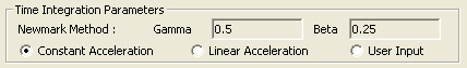
Newmark Method: Newmark Method is used to numerically integrate kinetic equations in direct integration. The related parameters, Gamma and Beta are entered. Three methods exist for input. Among them, Constant Acceleration is recommended, which always results in stable analysis.
Constant Acceleration: It is assumed that the acceleration of a structure remains unchanged during the time interval of each Time Step. The corresponding Gamma (=1/2) and Beta (=1/4) are automatically entered. Based on this assumption, volatility of analysis results can be prevented irrespective of the value of Time Increment in the analysis of direct Integration.
Linear Acceleration: It is assumed that the acceleration of a structure varies linearly during the time interval of each Time Step. The corresponding Gamma (=1/2) and Beta (=1/6) are automatically entered. Based on this assumption, the analysis results may become unstable in the analysis of direct Integration when the value of Time Increment is bigger than 0.551 times the shortest period of the structure.
User Input: User directly enters the values of Gamma and Beta.
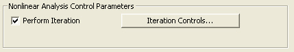
Nonlinear Analysis
Control Parameters
If Modal is selected
Enter the parameters necessary for nonlinear analysis when Nonlinear is selected in Analysis Type.

Perform Iteration: It performs convergence calculation by the Newton Raphson method.
Iteration Controls: Specify an Iteration Control method that determines the accuracy and convergence of a solution for nonlinear analysis.
Iteration Parameters: Specify Iteration Parameters that determine the accuracy and convergence of a solution for nonlinear analysis.
Permit Convergence Failure: It becomes inactivated for Nonlinear-Static Analysis.
Minimum Step Size: It is a Minimum value for Sub-steps, which are segmented from each analysis Time Step. If convergence calculation by the Newton Raphson method is used, but does not satisfy the Convergence Criteria even after reaching the maximum number of iterations, it automatically divides the time step into smaller sub-steps. The Minimum Sub-step Size limits the time interval between the sub-steps.
Maximum Iteration: The maximum number of iterations per each Sub-step for analysis. If Modal is selected in Analysis Method, Fast Nonlinear Analysis Algorithm developed by E. L. Wilson is used for iterative analysis. If Direct Integration is selected, the Newton Raphson iterative method is used. The maximum number of iterations is recommended to be less than 10. A large value may lead to a long analysis time.
Convergence Criteria: Define the convergence criteria for nonlinear time history analysis.
midas provides Displacement Norm, Force Norm and Energy Norm, which are used for the acceptance criteria for convergence in the iterative analysis process. Multiple norms can be selected. When the modal superposition method is used, Displacement Norm and Force Norm can be applied. For the direct integration method, all the 3 Norms can be used.
Boundary Nonlinear Analysis: Specify a convergence method that determines the accuracy and convergence of a solution for boundary nonlinear analysis.
Runge Kutta Method: Expand the increment time in a Taylor series to solve the differential equations.
Fehlberg Method (Stepsize sub-division for Non-convergence Control)
Cash-Karp Method (Adaptive Stepsize Control)
If Direct Integration is selected
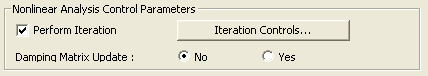
Perform Iteration: It performs convergence calculations by the Newton Raphson method.
Damping Matrix Update: When Direct Integration is used in nonlinear time history analysis, check whether to continuously update the element damping matrix based on the change in stiffness. If it is unchecked, the initial stiffness of the elastic state is used for the element damping matrix. If it is checked on, the element damping matrix is calculated using the presently modified stiffness. This menu only activates for Mass and Stiffness Proportional and Element Mass & Stiffness Proportional.
Iteration Controls: Specify an Iteration Control method that determines the accuracy and convergence of a solution for nonlinear analysis.
Iteration Parameters: Specify Iteration Parameters that determine the accuracy and convergence of a solution for nonlinear analysis.
Permit Convergence Failure: When Displacement/Force/Energy diverges between the Steps specified by the user, midas Gen automatically divides the steps and reanalyzes the model. If divergence still continues, the analysis proceeds unconverged to the next step if Permit Convergence Failure is checked on. Analysis results may contain some margin of error, but the unconverged results still may be helpful to understand the approximate behavior of the overall structure or to identify the cause of such divergence. Results obtained using this option can be unconverged, especially when the change of stiffness is significant due to nonlinear behavior. The time step should be reduced in such cases.
Minimum Step Size: It is the Minimum value for Sub-steps that are segmented from each analysis Time Step. If the convergence calculation by Newton Raphson method is used, but does not satisfy the Convergence Criteria even after reaching the maximum number of iterations, it automatically divides the time step into smaller sub-steps. The Minimum Sub-step Size limits the time interval between the sub-steps.
Maximum Iteration: It is the maximum number of iterations per each Sub-step for analysis. If Modal is selected in the Analysis Method, Fast Nonlinear Analysis Algorithm developed by E. L. Wilson is used for iterative analysis. If Direct Integration is selected, the Newton Raphson iterative method is used. The maximum number of iterations is recommended to be less than 10. If the number of iterations is large, considerable time may be required for analysis.
Convergence Criteria: Define the convergence criteria for nonlinear time history analysis.
midas Gen provides Displacement Norm, Force Norm and Energy Norm, which are used for the acceptance criteria for convergence in the iterative analysis process. Multiple norms can be selected. When the modal superposition method is used, Displacement Norm and Force Norm can be applied. For the direct integration method, all the 3 Norms can be used.
Boundary Nonlinear Analysis: Specify a convergence method that determines the accuracy and convergence of a solution for boundary nonlinear analysis.
Runge Kutta Method: Expand the increment time in a Taylor series to solve differential equations.
Fehlberg Method (Stepsize sub-division for Non-convergence Control)
Cash-Karp Method (Adaptive Stepsize Control)
If Static is selected
Perform Iteration: It performs convergence calculations by the Newton Raphson method.
Iteration Controls: Specify an Iteration Control method that determines the accuracy and convergence of a solution for nonlinear analysis.
Iteration Parameters: Specify Iteration Parameters that determine the accuracy and convergence of a solution for nonlinear analysis.
Permit Convergence Failure: When Displacement/Force/Energy diverges between the Steps specified by the user, midas Gen automatically divides the steps and reanalyzes the model. If divergence still persists, the analysis proceeds unconverged to the next step if Permit Convergence Failure is checked on. Analysis results may contain some margin of error, but the unconverged results still may be helpful to understand the approximate behavior of the overall structure or to identify the cause of such divergence. Results obtained using this option can be unconverged, especially when the change of stiffness is significant due to nonlinear behaviors. The time step should be reduced in such cases.
Max. Number of Substeps:
Maximum Iteration: It is the maximum number of iterations per each Sub-step for analysis. If Modal is selected in Analysis Method, Fast Nonlinear Analysis Algorithm developed by E. L. Wilson is used for iterative analysis. If Direct Integration is selected, the Newton Raphson iterative method is used. The maximum number of iterations is recommended to be less than 10. If the number of iterations is large, considerable time may be required for analysis.
Convergence Criteria: Define the convergence criteria for nonlinear time history analysis.
midas Gen provides Displacement Norm, Force Norm and Energy Norm, which are used for the acceptance criteria for convergence in the iterative analysis process. Multiple norms can be selected. When the modal superposition method is used, Displacement Norm and Force Norm can be applied. For the direct integration method, all the 3 Norms can be used.
Boundary Nonlinear Analysis: Specify a convergence method that determines the accuracy and convergence of a solution for boundary nonlinear analysis.
Runge Kutta Method: Expand the increment time in a Taylor series to solve differential equations.
Fehlberg Method (Stepsize sub-division for Non-convergence Control)
Cash-Karp Method (Adaptive Stepsize Control)
Note 1
In order to carry out a time history analysis, the required data
related to Eigenvalue analysis
or Ritz vector analysis must be entered in Eigenvalue
Analysis Control. In the case of Eigenvalue analysis, the
number of eigenvalues, the range of natural frequencies to be
considered, the maximum number of repetitions for the eigenvalue
calculation, the subspace dimension, the convergence tolerance,
the Frequency Shift for a rigid body motion, etc. must be entered.
In the case of Ritz Vector analysis, specify the starting load
vectors and the number of Ritz Vectors to be generated for each
starting load vector.
Note 2
During Nonlinear Static or Nonlinear Time History Analyses, the section can completely fail upon reaching the ultimate state. This is because all the tension rebars yield or the concrete in the compression zone is rapidly transferred to the Softening state having a negative modulus of elasticity.
Even in case the time history analysis diverges, the result before the divergence can be checked in post-processing.
![]() Revision of Gen 2015 (v1.1)
Revision of Gen 2015 (v1.1)