Analysis: Analysis Option
![]()
Function
Assign the static analysis method and the size of RAM to be used for the analysis.
Call
Analysis > Analysis Option
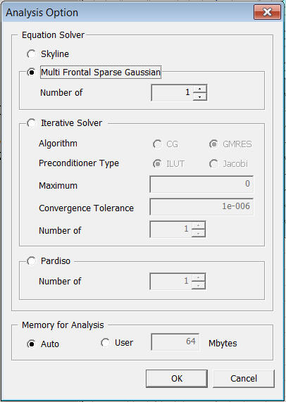
<Analysis Option>
Solver
Select the analysis solver be performed. All solvers are able to handle symmetric and non-symmetric analysis.
Skyline
This
method is most widely adopted in structural analysis programs. The method
is applicable irrespective of the type of analysis, the scale of the model
and the system settings. The Skyline solver can
perform analysis types that are Symmetric and initiates the Non-symmetric
Multi Frontal Sparse Gaussian solver for Non-symmetric types.
Multi Frontal Sparse Gaussian Solver
The high performance Multi-Frontal Sparse Gaussian Solver (MFSGS) is one of the latest addition to the group of MIDAS solvers. The MFSGS uses an optimum frontal division algorithm to minimize the number of calculations for simultaneous linear equations. The Multi Frontal Sparse Gaussian Solver is capable of handling analysis types that are Symmetric and Non-Symmetric.
Number of threads
Iterative Solver
Iterative
solver efficiently handles a large scale model. The basic principle of
Iterative solver is to approximate  to determine
  in
in  .
.
The following options should be specified for effective usage of Iterative Solver.
Algorithm
Conjugate Gradient Method(CG)
Conjugate Gradient Method (CG) is used when the stiffness matrix is symmetrically positive definite, and the most of structural analyses falls under this method. If the stiffness analysis of analyzing model becomes nonsymmetrical, the program will switch automatically to the GMRES method.
Generalized Minimum Residual Method(GMRES)
Generalized Minimum Residual Method (GMRES) can solve the problem when the stiffness matrix is not only indefinite but also nonsymmetrical. Therefore, this method is mostly used to handle specific nonlinear problems
For each algorithm, user can choose within a couple of methods to determine Preconditioner.
Preconditioner Type
Incomplete LU with drop-tolerance (ILUT)
By
default DIANA applies Incomplete LU-decomposition preconditioning, generally
known as ILU preconditioning, see Meijerink & Van Der Vorst [3]. The
idea of ILU preconditioning is to approximate the system matrix K by the
product of a lower diagonal matrix L and an upper matrix U  , to
, to  .
.
If the factorization is carried out exactly, we get a direct solution method. The disadvantage of the exact factorization is that fill-in occurs: the matrices L and U contain far more non-zero entries than the original matrix K . In the ILU approximation we try to restrict the fill-in of L and U . First we limit the fill to the sparsity pattern of K,
|
|
|

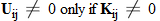
The ILU decomposition is uniquely defined by
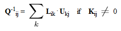
If the setup of Q fails, or if the subsequent iteration does not converge, we improve the preconditioner by allowing more fill-in. Therefore we use a drop-tolerance strategy: non-zero elements are only included in the incomplete factors if they are larger than a given threshold parameter (ILUT, see Saad [4]). This threshold parameter is determined adaptively: we decrease it until the iteration has converged. We notice that we obtain the exact factorization if the drop tolerance is small enough.
Jacobi Preconditioner
The most simple and probably the most widely used preconditioning technique is to scale the stiffness matrix with a diagonal matrix D . For problems with a diagonally dominant stiffness matrix the choice D equal to diag(K) , and hence Q equal to the inverse of diag(K), is both natural and good. This preconditioner is known as Jacobi preconditioning or diagonal scaling. .
Maximum Iteration
Specify the number of iterations until the analysis converges. When user defines the value to 0 (default setting), the program sets the maximum iteration to one fourth of total degrees of freedom.
Convergence Tolerance
Using the following condition, the program checks whether the finite element equation has converged to a solution or not.
where,
 : convergence tolerance
Number of
Specify maximum number of iterations.
PARDISO
Intel Math Kernel Library (Intel MKL) provides a direct sparse solver PARDISO which can be used for solving real symmetric and structurally symmetric sparse linear systems of equations.
The PARDISO solver shows both a high performance and memory efficient usage for solving large sparse symmetric and unsymmetric linear systems of equations by shared multiprocessors. The solver uses a combination of left- and right-looking supernode techniques, refer to [1] and [2]. For sufficiently large problems, the scalability of the parallel algorithm is nearly independent of the shared-memory multiprocessing architecture and a speedup of up to five using eight processors has been observed.
Memory for Analysis
Enter when the analysis is to be performed using only a part of the memory in the system.
Auto
If Auto
is selected, the program uses appropriate memory for the analysis after
it determines the state of memory in the computer.
User
The user defines the memory usage for analysis.
Notes
During the analysis, GTS solver creates several temporary files on the hard disk. It is recommended to have at least 3 gigs of available hard disk space.
[1] SCHENK, O.
Scalable Parallel Sparse LU Factorization Methods on Shared Memory Multiprocessors.
PhD thesis.
[2] SCHENK, O., GARTNER, K., AND FICHTNER, W.
Efficient Sparse LU Factorization with Left-right Looking Strategy on Shared Memory Multiprocessors.
BIT 40, 1 (2000), 158-176.
[3] MEIJERINK, J. A., AND VAN DER VORST, H. A.
An iterative solution method for linear systems of which the coefficient matrix is a symmetric M-matrix.
Math. Comp. 31 (1977), 148-162.
[4] SAAD, Y.
ILUT: a dual threshold incomplete ILU factorization.
Numerical Linear Algebra with Applications 1 (1994), 387-402.