Used to create a time load function for time history analysis directly. The static load and force (pressure load) is defined by applying a time forcing function. The applicable time function data type for dynamic nodal loads are ‘Force’, ‘Moments’ and, for dynamic surface loads, ‘Normal’. In addition, the reference function can be applied to define a linear/non-linear distributed dynamic load that changes with position. Generally it is used to define vibration, driving, blast and railway movement loads. The arrival time can be set to simulate the delay time.

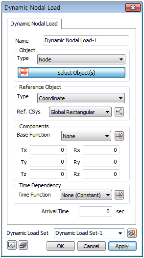
Select the node where the load will be applied and specify the direction. The load size is applied by multiplying the time function (load size by time) and each load component (scale factor).

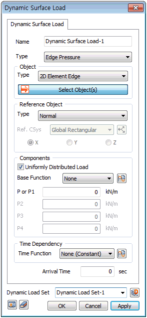
[Object]

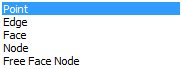
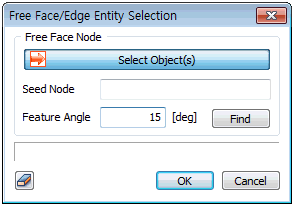
The applied load is defined on the node , but the selection target can also be set as a geometry shape (edge, surface etc.) or using auto-select free face nodes. For a line or surface, the selected shape must have been used for element creation and the force is applied to all nodes in the specified direction/size. For free face nodes, select a free face node and all points that make contact with the node-containing element at an angle smaller than the specified angle (feature angle) will be automatically selected.

[Reference Object]

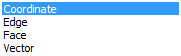
The load direction can be set using different methods. The default input reference is the Global rectangular(cylindrical) coordinate axis. Geometry shapes (Edge and Surface) can be selected as a  reference direction. Selecting 'Line' or 'Surface' displays the coordinate system of the selected shape and the load is set with reference to that system. 'Vector' is used to specify the load direction using X,Y,Z vector components.

[Components]

Input the load scale factor according to the set direction. Generally, the load size is pre-defined as a time variant value in the time function, and if the maximum ratio value is defined as 1, the actual load size is input in the time function. A positive (+) value applies the load in the set direction and a negative (-) value applies the load in the opposite direction to the set direction. The load size change, depending on the coordinate value increase in the global coordinate system (GCS), can be defined using a reference function. Here, the input value is multiplied by the function value for application.

[Time Dependency (Time function)]

Define the load size change with respect to time.

Select the  button to add (select) a time forcing function. It can only be applied when the time forcing function data type is 'Acceleration', 'Velocity', 'Displacement', ‘Force’ and ‘Moments’.

Methodology (Dynamic Surface)

Dynamic surfaces are input as the distributed load change with respect to time on the element face or edge. It can be used on 2D or 3D elements and the input direction can be specified as an arbitrary coordinate axis direction, arbitrary vector direction or normal direction.

[Components]

Input the load scale factor according to the set direction. The uniform or linear/non-linear distributed load can be defined. A positive (+) value applies the load in the set direction, while a negative (-) value applies the load in the direction opposite of the set direction. The load size change, depending on the coordinate value increase in the global coordinate system (GCS), can be defined using a reference function. Here, the input load component is multiplied by the function value for application.

[Time Dependency (Time function)]

Define the load size change with respect to time.

Select the   button to add (select) a time forcing function. It can only be applied when the time forcing function data type is ‘Normal’. ‘Normal’ functions are dimensionless and have no units. Hence, if the pressure load size is directly entered, only the scale factor is input for the load component. If the maximum ratio value is defined as 1, the actual load size is input.