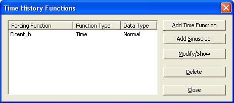
Time Forcing Functions

Assign time forcing functions for time history analyses.

From the Main Menu select Load > Time History Analysis Data > Time Forcing Functions.

Select Time History Analysis > Time Forcing Functions in the Menu tab of the Tree Menu.

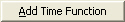
Time History Functions dialog box

Enter new or additional time forcing functions

Click when the time forcing function is of random type or a walking load. Click when the time forcing function is sinusoidal.

Modify previously entered time forcing functions

Select a time forcing function from the list in the dialog box and click .

Delete previously entered time forcing functions

Select a time forcing function from the list in the dialog box and click .

Data entry method by clicking .

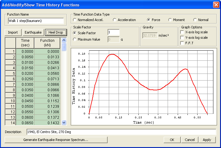
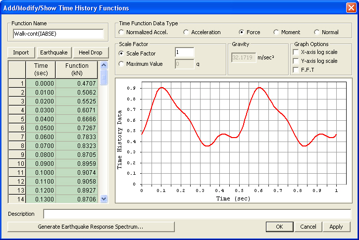
Add/Modify/Show Time History Functions dialog box

Function Name

Enter the name of the time forcing function. The name is used in "Dynamic Nodal Loads" and "Ground Acceleration" which are data entry features of the time history forcing functions. In the case of a walking load or earthquake data, the name may be automatically selected.

Time Function Data Type

Select a type of Time Function Data.

Normalized Accel.: Values obtained through Time History Accelerations divided by the gravitational acceleration

Acceleration: Time history accelerations

Force

Moment

Normal: Non-dimensional

Force or Moment is selected to enter the time history loads as dynamic nodal loads in the "Dynamic Nodal Loads" function.

Normalized Accel. or Acceleration is selected to enter the time history loads as ground accelerations in the "Ground Acceleration"

function. Normal is selected to enter the time history loads as time dependent static loads in the "Time Varying Static Loads"

function.

Scale Factor

Specify a multiplier for Time History Data.

If the user modifies Time Function Data Type while a time history load has been entered, only the units of the data will be changed, and the data (corresponding values) themselves will not be changed to the units of the revised Data Type. By using Scale Factor, all the values of the time history data can be simply revised.

For example, when the user enters 0.1g in Normalized Acceleration and subsequently changes the units to Acceleration, the magnitudes of the values will not be changed but remain as the entered value, 0.1m/s^2. In order to change 0.1g in the units of m/s^2, 9.8 needs to be entered in the Scale Factor, since 0.1g=0.98m/s^2.

Gravity

Display the applied acceleration of gravity, which may be revised in Model > "Structure Type".When the time forcing function is entered using the Normalized Acceleration type, it will be divided by the Gravitational Acceleration for analysis.

Graph Options

Specify whether or not to produce Graph in Log Scale.

Description

Enter a brief description of Time History Function.

For convenience, MIDAS/Gen supports the following 3 data entry methods:

1. Save and retrieve frequently used time history loads in and from files

2. Access the built-in time history loads from the database

3. The user directly enters the time function data

Save and retrieve frequently used time history loads in and from files

Enter the time history loads by reading previously created files. The data are saved with '.sgs' or '.thd' extension and are written according to the following formats.

'fn.sgs' file format

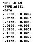
'fn.thd' file format (User's entries)

(Example of fn.thd input)

Access the built-in time forcing functions from the MIDAS/Gen database

Create time history loads by reading earthquake records from the database.

There are 32 types of built-in seismic accelerations in the database.

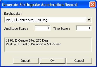
Generate Earthquake Acceleration Record dialog box

Create time history loads automatically according to the specified weight of a walker, walking speed and time intervals.

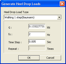
 Generate Heel Drop Loads dialog box

Applicable walking loads are as follows:

Walking 1 step (Baumann)

Baumann K. Bachmann H. suggested a loading time history based on a one step of a pedestrain, which was subsequently idealized to reflect the weight of the pedestrain and the walking speed.

Walking - continuous (IABSE)

Baumann's walking load has beenfurther refined by IABSE (International Association for Bridge and Standard Engineering), AIPC (Association Internationale des Ponts et Charpentes) and IVBH (Internationale Vereinigung fur Bruckenbau Hochbau).

: Weight of pedestrain

= 0.4 , fs = 2.0 Hz

= 0.5, fs = 2.4 Hz

==0.1

= =

Note
IABSE's loading time history premises that a pedestrain continuously walks on the same location. This is not applicable for "walking". The results may be relible for the walking frequency range of 2.0 ~ 2.4 Hz and the number of repetition of more than 2.

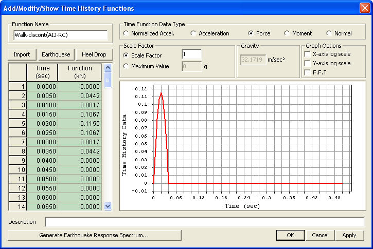
Walking - discont.(AIJ)

The forcing function premises that the walking load is expressed as the impact energy , 0.3 kgf·sec, which exerts over 0.04 second.

unit: kgf

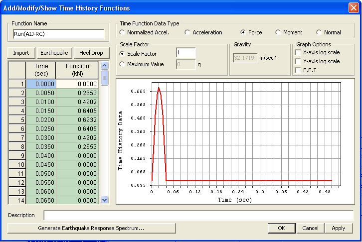
Running (AIJ)

The forcing function for running load is similarly derived as for walking load except for the impact energy of 1.8 kgf·sec.

unit: kgf

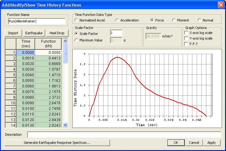
Running-(Allen & Rainer)

Note
Walking vibration have been known to occur in the frequency range of 1.5 ~ 2.5 Hz.
Depending on the natural frequency of the floor structure, the engineer must exercise caution to apply walking frequencies that result in maximum response.

Enter directly the time forcing functions in the entry fields in the Add/Modify/Show Time History Functions dialog box

The user directly enters the time and the values of the time forcing function in the entry fields to the left of the dialog box.

Data entry method by clicking . 

Add/Modify/Show Time History Functions dialog box

Function Name

Enter the name of the time forcing function. The name is used in "Dynamic Nodal Loads" and "Ground Acceleration" which are data entry features of the application of the time history forcing functions.

Time Function Data Type

Assign the type of data to be entered.

Normalized Accel.: Values obtained by dividing the time history acceleration by the acceleration of gravity

Acceleration: Time history acceleration

Force: Load (force)

Moment: Moment

When Force or Moment is assigned, the time forcing function is used to enter the "Dynamic Nodal Loads" and when Normalized Accel. or Acceleration is assigned, it is used to enter the "Ground Acceleration".

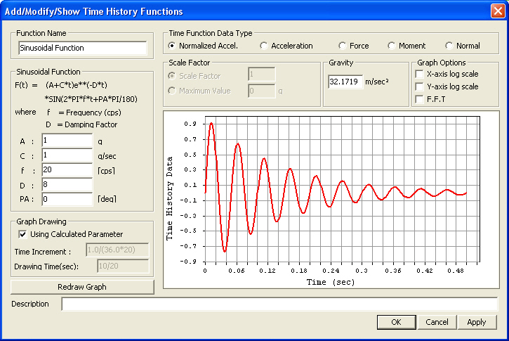
Parameters constituting the Sinusoidal Functions

A, C are constants, f is the frequency of excitation, D is the Damping Factor, PA is the Phase Angle.

When the time forcing function is entered in the form of a harmonic function, specify the parameters required in Sinusoidal Function. Click Redraw Graph to display the graph of the forcing function to the right and click to save the time forcing function.