Inelastic Hinge Properties
| ||||||||||||||||||||||||||||||||||||||||||||||||||||||||||||||||||||||||||||||||||||||||||||||||||||||||||||||||||||||||||||||||||
|
| ||||||||||||||||||||||||||||||||||||||||||||||||||||||||||||||||||||||||||||||||||||||||||||||||||||||||||||||||||||||||||||||||||
|
| ||||||||||||||||||||||||||||||||||||||||||||||||||||||||||||||||||||||||||||||||||||||||||||||||||||||||||||||||||||||||||||||||||
|
Add, modify or delete inelastic hinge properties.
Inelastic hinges are applied to inelastic time history analysis only.
The Spring Type hinge defined in General Link Properties can be used for pushover analysis if the inelastic hinge properties are assigned to the hinge. | ||||||||||||||||||||||||||||||||||||||||||||||||||||||||||||||||||||||||||||||||||||||||||||||||||||||||||||||||||||||||||||||||||
|
| ||||||||||||||||||||||||||||||||||||||||||||||||||||||||||||||||||||||||||||||||||||||||||||||||||||||||||||||||||||||||||||||||||
|
| ||||||||||||||||||||||||||||||||||||||||||||||||||||||||||||||||||||||||||||||||||||||||||||||||||||||||||||||||||||||||||||||||||
|
| ||||||||||||||||||||||||||||||||||||||||||||||||||||||||||||||||||||||||||||||||||||||||||||||||||||||||||||||||||||||||||||||||||
|
From the Main Menu Select Model > Properties > Inelastic Hinge Properties.
Select Geometry > Properties > Inelastic Hinge Properties in the Menu tab of the Tree Menu. | ||||||||||||||||||||||||||||||||||||||||||||||||||||||||||||||||||||||||||||||||||||||||||||||||||||||||||||||||||||||||||||||||||
|
| ||||||||||||||||||||||||||||||||||||||||||||||||||||||||||||||||||||||||||||||||||||||||||||||||||||||||||||||||||||||||||||||||||
|
| ||||||||||||||||||||||||||||||||||||||||||||||||||||||||||||||||||||||||||||||||||||||||||||||||||||||||||||||||||||||||||||||||||
|
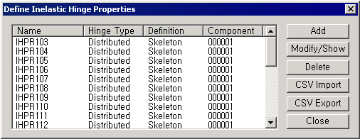
Define Inelastic Hinge Properties dialog box
CSV Export
Rows 12 ~ 29 are differently entered depending on the Input Type of Yield Properties.
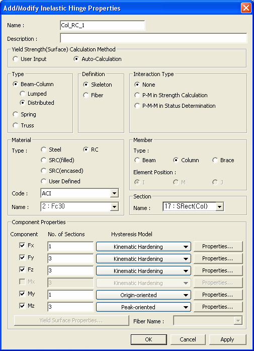
Add/ Modify Inelastic Hinge Properties dialog box
| ||||||||||||||||||||||||||||||||||||||||||||||||||||||||||||||||||||||||||||||||||||||||||||||||||||||||||||||||||||||||||||||||||
 to add
Inelastic Hinge Properties.
to add
Inelastic Hinge Properties. button and change the input.
 button.
 : Import
inelastic hinge properties saved in a CSV file.
: Import
inelastic hinge properties saved in a CSV file. : Export
inelastic hinge properties to a CSV file. Only the inelastic hinge properties
defined as User Type will be available for output. Only the inelastic
hinge properties defined as
: Export
inelastic hinge properties to a CSV file. Only the inelastic hinge properties
defined as User Type will be available for output. Only the inelastic
hinge properties defined as  : Close Inelastic
Hinge Property dialog box.
: Close Inelastic
Hinge Property dialog box. 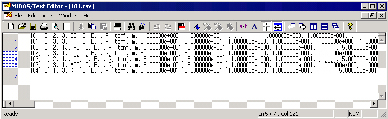
|
|
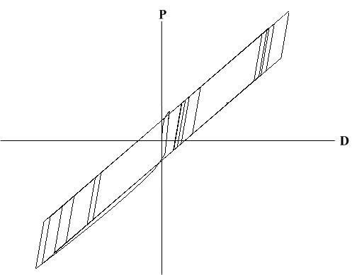
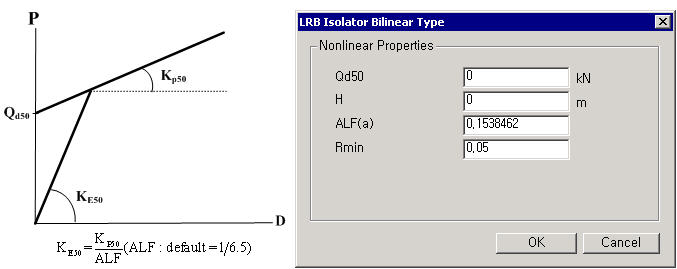
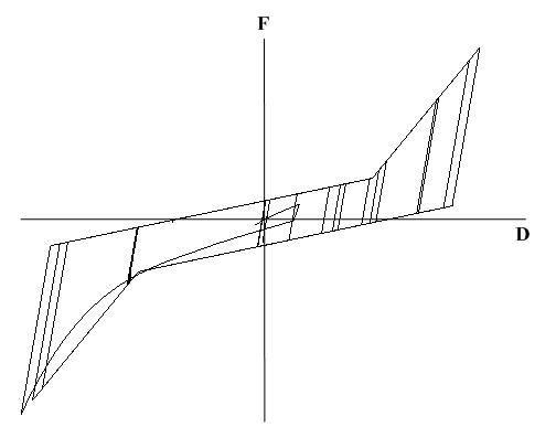
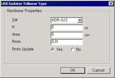
H: layer thickness Area: contact area R_min: initial shear strain (Default 0.01) SW: bearing type 1: HDR-G12 (default) LRB Isolator Trilinear type hysteresis model
can be applied to General Link of Spring Type only. |
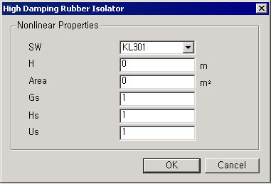
 High
Damping Rubber Isolator type hysteresis model
High
Damping Rubber Isolator type hysteresis model
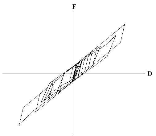
High Damping Rubber Isolator Type hysteresis model
|
|
H: layer thickness Area: contact area R_min: initial shear strain (Default 0.01) SW: bearing type 1: KL301 (default) Gs: coefficient multiplied to shear elastic modulus (default : 1.0) Hs: coefficient multiplied to equivalent damping (default : 1.0) Us: coefficient multiplied to yield loading
property coefficient High Damping Rubber Isolator Type hysteresis
model can be applied to General Link of Spring Type only. |
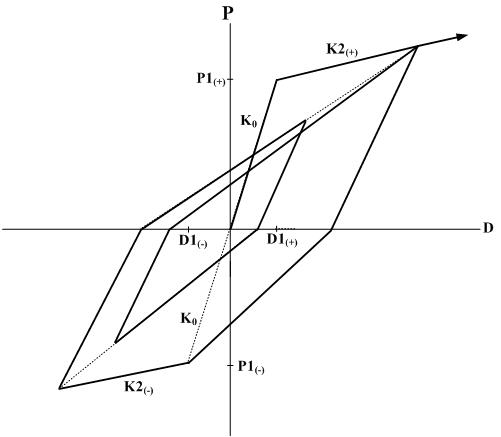
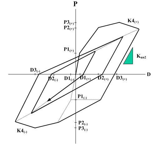
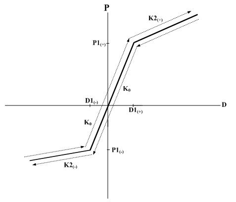
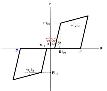
Slip
Bilinear
Type hysteresis model
|
Slip Bilinear Type hysteresis model
|
|
|
Slip Bilinear/Tension Type hysteresis model
|
|
|
Slip Bilinear/Compression Type hysteresis model
|
|
|
*. When the initial Gap
| |
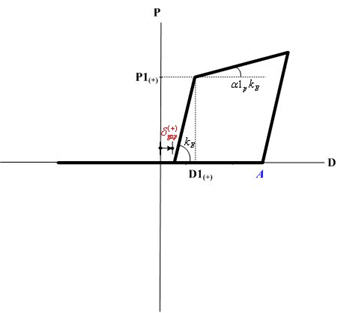
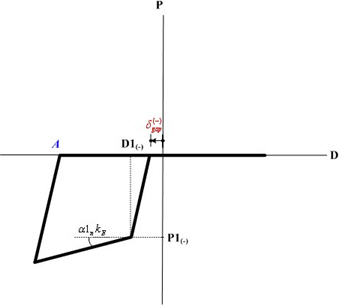
 is entered in the Slip Bilinear type hysteresis model, plastic
ratio (D/D1) is calculated by the equation
is entered in the Slip Bilinear type hysteresis model, plastic
ratio (D/D1) is calculated by the equation  .
.
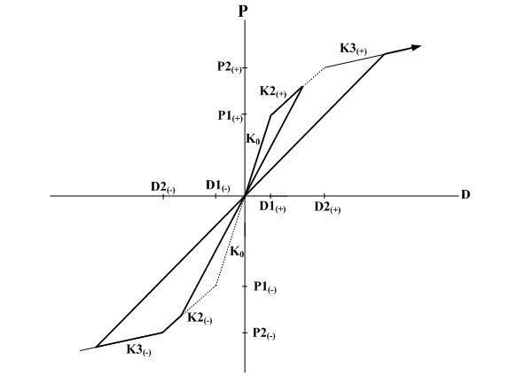
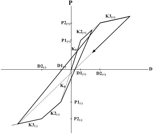
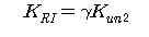
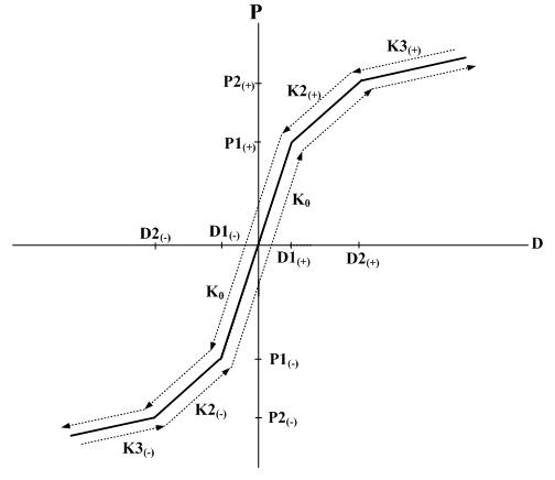
Slip
Trilinear
Type hysteresis model
|
Slip Trilinear Type hysteresis model
|
|
|
Slip Trilinear/Tension Type hysteresis model
|
|
|
Slip Trilinear/Compression Type hysteresis model
|
|
|
*. When the initial Gap (
| |
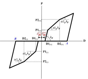
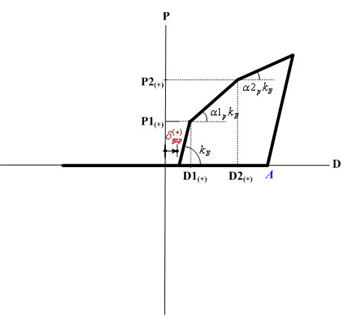
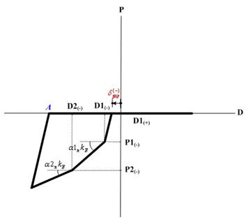
 ) is entered in the Slip Trilinear type hysteresis model,
plastic ratio (D/D1, D/D2) is calculated by the equation .
) is entered in the Slip Trilinear type hysteresis model,
plastic ratio (D/D1, D/D2) is calculated by the equation .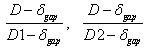
Note
When the Spring Type general link element is defined as inelastic hinge
for pushover analysis, all the hysteresis models provided by MIDAS/Gen
can be used.
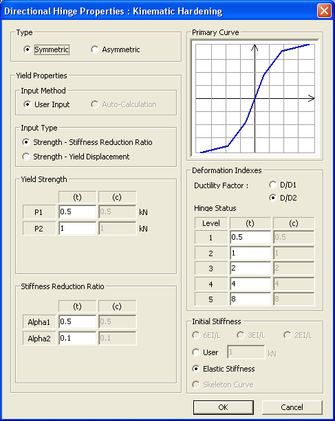
Directional Hinge Properties dialog box
 Type
Type
Select whether or not the skeleton curve is symmetrical. Non-symmetry of the curve can be applied to Yield Strength, Stiffness Reduction Ratio and Hinge Status. However, Kinematic Hardening Model does not permit non-symmetry of Stiffness Reduction Ratio due to its characteristics.
Yield Properties
Input Method
User Input: User defines the Yield Properties.
Auto Calculation: The Yield Properties are automatically calculated.
Input Type
Strength-Stiffness Reduction Ratio: Yield Properties are defined by specifying Strength-Stiffness Reduction Ratio.
Strength-Yield Displacement: Yield Properties are defined by specifying Strength-Yield Displacement.
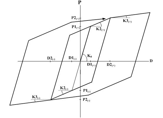
Yield Strength
Yield strength is specified. It is user defined based on material and section properties. The user specifies positive (+) values regardless of tension (t) or compression (c). The program treats compression as negative (-) internally.
P1: P1 represents the first yield strength. If the Material Type is Steel or SRC (filled), the first yield represents the state in which the maximum bending stress of the section reaches the yield stress. If the Material Type is RC or SRC (encased), the first yield represents the state in which the maximum bending stress of the section reaches the cracking stress of concrete.
P2: P2 represents the second yield strength. If the Material Type is Steel or SRC (filled), the second yield represents the state in which the bending stress of the entire section reaches the yield stress. If the Material Type is RC or SRC (encased), the second yield represents the state in which the stress in the concrete section reaches the ultimate strength or the stress in reinforcing steel reaches the yield strength. In case of bending, the concrete stress is based on a rectangular stress block.
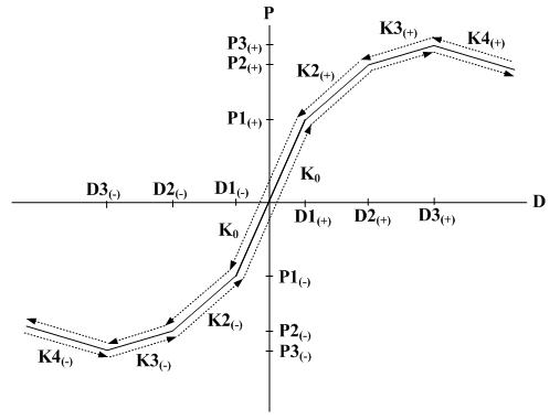
P3: P3 represents the third yield strength.
Stiffness Reduction Ratio
Enter the stiffness reduction ratios of a sloped skeleton curve when Strength - Stiffness Reduction Ratio is selected for Input Type.
α1: Ratio of stiffness immediately after the first yielding divided by the initial stiffness
α2: Ratio of stiffness immediately after the second yielding divided by the initial stiffness, which is defined when the skeleton curve is of Trilinear or Tetralinear type.
α3: Ratio of stiffness immediately after the third yielding divided by the initial stiffness, which is defined when the skeleton curve is of Tetralinear type.
Yield Displacement
Enter the yield displacement of a sloped skeleton curve when Strength - Yield Displacement is selected for Input Type.
D1: first yield displacement component or deformation
D2: second yield displacement component or deformation, which is defined when the skeleton curve is of Trilinear or Tetralinear type.
D3: third yield displacement component or deformation, which is defined when the skeleton curve is of Tetralinear type.
Deformation Indexes
Data required for calculating the indexes, which represent the level of deformation of an inelastic hinge
Ductility Factor: Select a basis of calculating ductility. Depending on the selection by the user, ductility factor is calculated by dividing the current deformation by the first yield deformation or the second yield deformation
Hinge Status: Enter the reference ductility, which classifies the state of a hinge in 5 different levels. In case of a non-symmetric hinge, the hinge status level at each time step is determined by the larger of the positive (+) and negative (-) levels. Level-1 (0.5) signifies the elastic status and Level-2 (1) signifies the yield status. Level-3 (2), Level-4 (4) and Level-5 (8) represent the level of ductility of each member. In analysis results, the status is presented in blue, green, yellowish light green, orange and red colors.
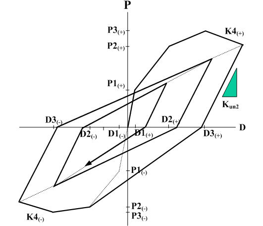
Initial Stiffness
The initial stiffness used in inelastic analysis is either selected or entered by the user.
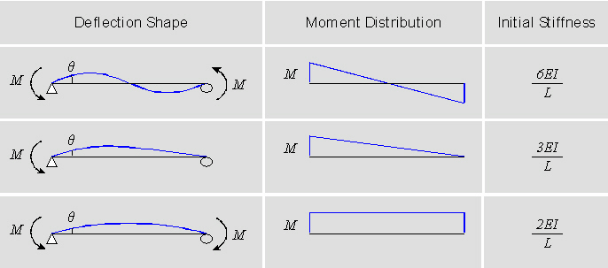
The selection of initial stiffness is founded on the premises of the longitudinal distribution of bending moment. If the bending moments, which are assumed to be linearly distributed, are the same in magnitude with opposite signs at both ends, select 6EI/L. If one end is 0, select 3EI/L. If the magnitudes and the signs are identical, select 2EI/L.
6EI/L , 3EI/L, 2EI/L: Provided that the inelastic hinge is of a lumped type for the bending moment component, the initial stiffness is selected on the basis of the longitudinal distribution of bending moment. This cannot be selected in case of Distributed Type and Spring Type.
6EI/L: when end values of linearly distributed bending moment are identical in magnitude but in opposite directions
3EI/L: when one end is 0
2EI/L: when the magnitudes and signs of end values are identical
User: the user directly enters the initial stiffness if the Input Type is Strength - Stiffness Reduction Ratio.
Elastic Stiffness: elastic stiffness of a member is used as the initial stiffness for inelastic analysis.
Skeleton Curve: when Strength - Yield Displacement is selected for the Input Type, the ratio of the user specified yield strength and yield displacement is used as the initial stiffness.
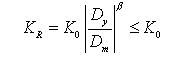
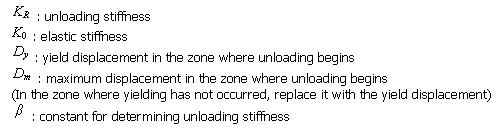
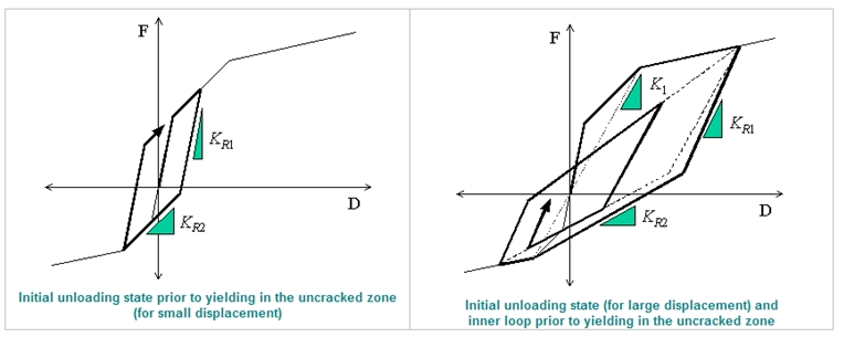
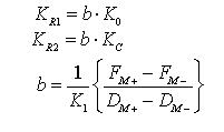
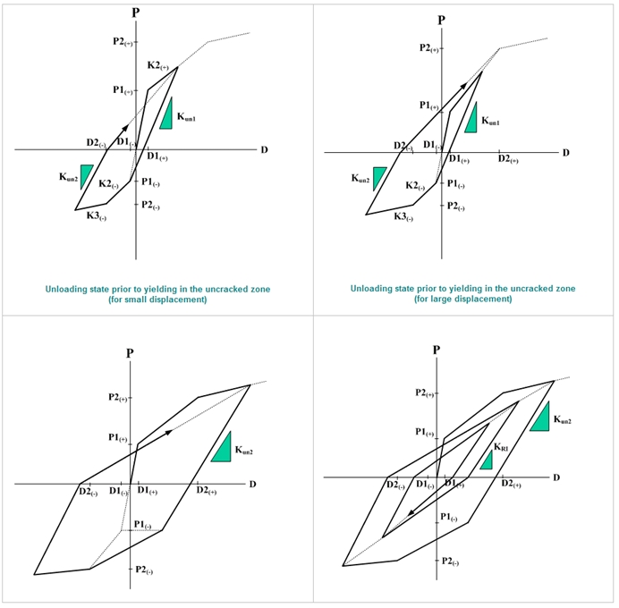
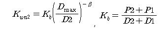
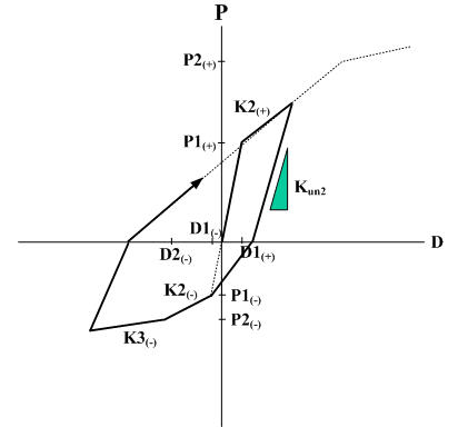
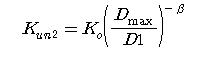
Unloading Stiffness Parameter
Exponent in Unloading Stiffness Calculation: This is an option used to determine the unloading stiffness of the outer loop used in the Clough and Takeda type models among hysteresis models of skeleton curves. This is used to reflect the effect of reduction in stiffness, which occurs as the deformation progresses after yielding. The unloading stiffness is determined by the elastic stiffness reduced by the yield displacement and maximum displacement in the zone where unloading begins and the exponent entered here.
Inner Loop Unloading Stiffness Reduction Factor: This is used to determine the unloading stiffness of the inner loop. The inner loop is formed when unloading occurs before reaching the target point on the skeleton curve while reloading after the loading sign changes in the process of unloading. The unloading stiffness of the inner loop is calculated by multiplying the unloading stiffness of the outer loop by the reduction ratio for the unloading stiffness of the inner loop.
Yield Surface Properties
If "P-M in Strength Calculation" or "P-M-M in Status Determination" is selected in Interaction Type, enter the data related to P-M interaction curve and corresponding 3-dimentional yield surface.
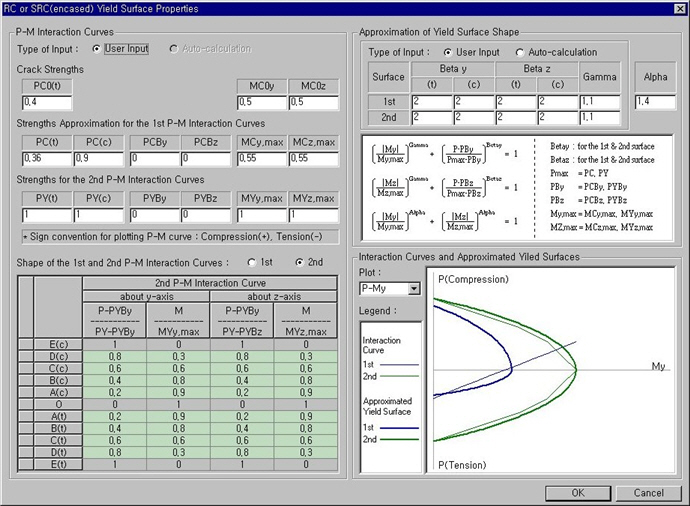
Yield Surface Properties dialog box
P-M Interaction Curves
Enter the P-M interaction curve data required to calculate 3-dimensional yield surfaces. All strength values must be entered with positive sign. Sign convention for plotting P-M curve is positive for compression and negative for tension.
Type of Input: Two input methods, user defined and auto-calculation based on material and section type, are supported to define the variables below. If some items are auto-calculated and the remainder is to be user defined, Auto-calculation should be performed first, and then necessary items can be modified after converting to User Input.
Crack Strengths
The following three items are required only if the Material Type is of
RC or SRC (encased). All the numerical values are entered as positive.
NC0(t): Cracking strength due to pure tension force
MC0y: Cracking strength of a section subject to moment about y-axis without the presence of axial force
MC0z: Cracking strength of a section subject to moment about z-axis without the presence of axial force
The following 12 items are required irrespective of the Material Type. But for RC and SRC (encased) sections, approximate NC(t), NC(c), NCBy, NCBz, MCy,max and MCz,max are either entered or auto-calculated on the basis of NC0(t), MC0y and MC0z. All the numerical values are entered as positive.
Strengths for the 1st P-M Interaction Curves
NC(t): First yield strength subject to pure tension force
NC(c): First yield strength subject to pure compression force
NCBy: Axial force at the time of balanced failure in the first yield interaction curve for the y-axis moment of the section
NCBz: Axial force at the time of balanced failure in the first yield interaction curve for the z-axis moment of the section
MCy,max: Maximum bending yield strength in the first yield interaction curve for the y-axis moment of the section
MCz,max: Maximum bending yield strength in the first yield interaction curve for the z-axis moment of the section
Strengths for the 2nd P-M Interaction Curves
NY(t): Second yield strength subject to pure tension force
NY(c): Second yield strength subject to pure compression force
NYBy: Axial force at the time of balanced failure in the second stage yield interaction curve for the y-axis moment of the section
NYBz: Axial force at the time of balanced failure in the second yield interaction curve for the z-axis moment of the section
MYy,max: Maximum bending yield strength in the second yield interaction curve for the y-axis moment of the section
MYz,max: Maximum bending yield strength in the second yield interaction curve for the z-axis moment of the section
Shape of the 1st and 2nd P-M Interaction Curves:
Input the P-M interaction curve shapes. The shape of an interaction curve is defined by coordinates of 11 points among which the furthermost extreme coordinates for tension, compression and flexure are fixed to 0 or 1. Only the remaining 8 points are thus entered. If Material Type is RC or SRC (encased), the interaction curve for the first yield is of a linear shape and as such input is unnecessary. In calculating or displaying the axial component of the coordinates, the sign convention is (+) for compression and (-) for tension.
Approximation of Yield Surface Shape
On the basis of P-M interaction curve, the parameters for 3-dimensional yield surface are either user defined or auto-calculated. If some items are auto-calculated and the remainder is to be user defined, Auto-calculation should be performed first, and then necessary items can be modified after converting to User Input. In case of Alpha, only user defined entry is possible. The value of each parameter is used in the equation of yield surface displayed in the dialog box.
Beta y, Beta z, Gamma: Being the exponential powers of P-My or P-Mz interactions, different values can be entered for the first and second yields. For Beta y and Beta z on the other hand, two separate values representing the ranges of larger and smaller axial forces relative to the axial force at the time of balanced failure can be entered. Alpha: Exponential powers of My-Mz interactions for the first and second yields.
Alpha: Exponent for My-Mz interaction for 1st and 2nd yielding
Coupling of Axial Force & Bending Moments: Select an interaction relationship between the components of axial and biaxial moments. Basically it is assumed that axial force and biaxial moments are inter-related in evaluating the hinge status. Nevertheless, the relationship between the axial force and the biaxial moments can be assumed to be either independent or coupled in formulating the stiffness matrix.
Interaction Curves and Approximated Yield Surfaces
The P-M interaction curves entered by the user or calculated by material and section properties and the 3-dimensional yield surfaces composed from them are displayed. The yield surfaces are displayed by showing the outlines of projection on the reference plane. Through this can we then check how well the P-M interaction curves and the yield surfaces coincide.
Plot: Select an interaction curve or yield surface to be displayed. P-My, P-Mz or My-Mz can be selected.