Point spring

Create a spring with a constant stiffness on the selected node. The constraints on deformation and rotation with reference to the GCS are defined by the spring constant and damping coefficient. It is mostly used as a flexible support condition for ground or a constraint condition for dynamic analysis.

Matrix Spring

Has the same function as the Point spring. However, the spring constant for deformation and rotation can be directly input into a matrix when defining the characteristics.

Rigid links

Create a link element that connects 2 selected nodes. Select the first node (reference) and select multiple nodes that become the connection target. It is used to simulate the rigid behavior between 2 nodes under deformation and rotation and the constraint direction can be defined the with reference to the GCS.

Elastic link

Connect 2 nodes with a spring that has a constant stiffness. Select the first node (reference) and select another node to create the link. Like the point string, the property is defined by the constant stiffness to deformation and rotation.

Interpolation

This function simulates the behavior of the standard (reference) node by weighing the average behavior of the selected nodes. It restricts the movement between connected nodes, similar to the rigid link. However, the interpolation element allows the relative behavior of a node due to movement at multiple different nodes. Hence, the average behavior at the multiple other nodes determines the movement of the reference node (dependent node).

Select the nodes to restrict and the degree of freedom, and then select the nodes to take the average values from. The weight of each node can be applied.

<Rigid link>                                  <Interpolation>

Surface spring

Create a point spring or elastic link by entering the spring stiffness per unit area at the support point of an element.

This is used to consider the flexible support condition of the ground during foundation analysis or underground structure analysis. Entering the spring stiffness per unit area automatically converts it to the spring or link acting on the node by considering the selected element area.

The surface spring inputs are as follows.

• Frame: Create a point spring or elastic link on a 1D element node. Input the width to calculate the support stiffness per unit length of a beam element.

• Planar: Create a spring or link by selecting a 2D element.

• Solid-Face: Specify an arbitrary surface on 3D Solid and create a spring or link at all nodes connected to that surface.  

• Element Edge: Select an outline of a 2D element and create a spring or link at the nodes connected to that outline.

The stiffness of the soil varies with depth. To define the varying stiffness with respect to space using the surface spring function of GTS NX,  the [Base Function] is to be used as the input.

The input elastic link per unit area is a way to define the spring constant. Other options are available, such as [Tension only] or [Compression only].

Ground surface spring

 - Auto generation of elastic/viscous boundary

This automatically creates the elastic/viscous boundary elements needed for dynamic analysis. Selecting a mesh automatically creates boundary conditions at the left/right/floor of the selected mesh and the spring constant is automatically calculated from the material/characteristics assigned to the element.

For dynamic analysis, the bottom of the model (floor surface) is often assigned a fixed condition (displacement constraint) to simulate bedrock conditions. Check the [Fixed Bottom Condition] to set this condition more easily.

NOTE:  As ground surface spring stiffness values are calculated by elastic modulus, Poisson's Ratio and Unit Weight of Ground, this element type cannot be directly applied for constitutive soil models like D-min, Jardine, Modified Mohr-Coulomb, Hardening Soil (HSS), Ramberg-Osgood, GHE-S, and Hardin-Drnevich. This is because the above mentioned models do not have Elastic Modulus Input. In case of these soils, the ground reaction force coefficient or damping constant can be applied to a surface spring element.

• When using an Outcrop motion as an input motion at the base of the model, a rigid base boundary will not produce correct results. In such cases, we need to use the Complaint Base function. When the complaint base is used half of the input (downward motion) applied to the ground node is absorbed by the damper, and half is forwarded to the node of the main ground mesh. In the latest version, the user has the option to choose between Absorbent, Complaint Base, and Rigid Base.
 

How to create an elastic boundary element  

• The elastic spring is used as a ground boundary condition for Eigen value analysis and Response spectrum analysis.

• Creating an elastic spring can be hard for beginners and the elastic spring element can be created from the following steps.

1.Use the elastic modulus of the ground to compute  Kv0. (The Equation is shown below.)

Here, E0: Elastic modulus of the ground, a Coefficient depending on test condition

2. Re-calculate the Subgrade Reaction Modulus Kv(= Kh) using the computed Kv0.

Here,  

The area Av becomes the area where the subgrade reaction spring will be installed.

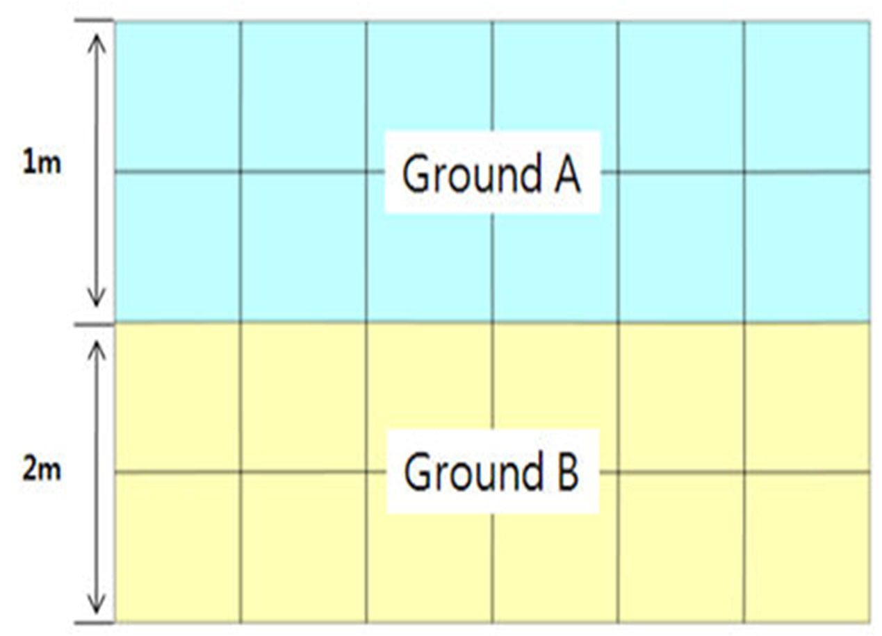
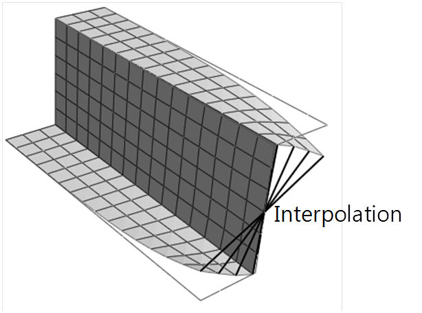
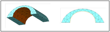
If the model exists like the following figure,

Area of Ground A is Av=1m(Left length of model)*1m(Unit width of 2D analysis)=1m2, Bv becomes 1m=100cm.

Using the same method, the unit width of Ground B is Bv=√(20000)cm=141.42136 cm.

Ultimately, the Subgrade Reaction Modulus K can be computed and a point spring is created on the node, considering the area of the element.

The spring coefficient of the floor (Z direction) is created with the same value as the X direction.

(Element length x Width (1m) = Cross sectional area, so only consider the effective length of the element.)

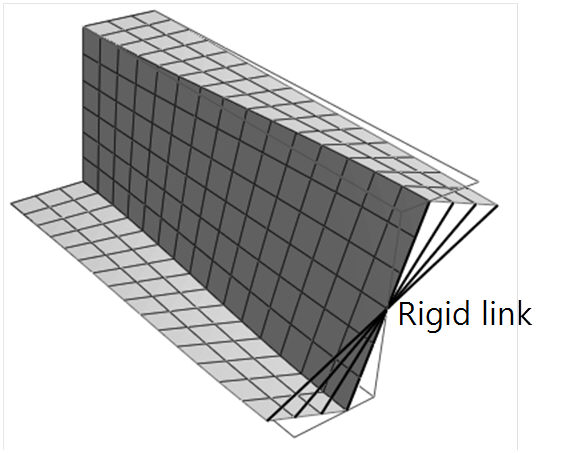
2 overlapping boundary elements are created where the ground and ground meet.

How to create a viscous boundary element

• The viscous boundary element required as a model boundary condition for time history analysis.

• The viscous boundary element can be created from the following steps.

1. Compute Cp, Cs

Cp, Cs can be calculated using the equation below.

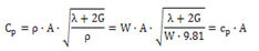
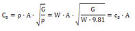
Here, , ,

λ : Bulk modulus, G : Shear modulus, E : Elastic modulus, ν : Poisson’s ratio, A : Cross-section area

2. The cross-section area is automatically considered until the surface spring is created, so only the Cp, Cs needs to be computed.

Multiplying the Cp, Cs (tonf•sec/m3 units) to the cross-section area eventually leads to the spring stiffness of the viscous boundary element in tonf•sec/m units.

The shaded cell parameters are the physical properties of the ground the user inputs during modeling and the Bulk modulus and Shear modulus are calculated using the Elastic modulus and Poisson’s ratio. Hence, there is no need to input additional values when creating a viscous boundary element.

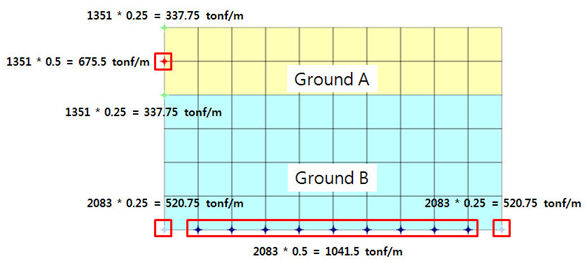
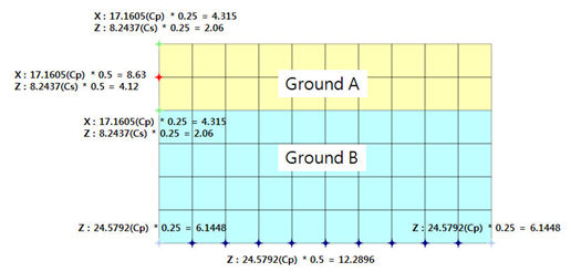
When creating the viscous boundary element automatically, the spring is automatically created by considering the element area (effective length*unit width) as shown below. Input the Cp value for the normal direction coefficient at the point of spring creation and input the Cs value for the parallel direction.

For example, the Cx of the spring coefficient created on the left/right of the model is the Cp of each ground and Cz becomes the Cs value. The bottom spring coefficient Cz becomes the Cp value.  

Gauging shell

Create a shell element to check the force and moment on the surface of a solid element structure. To create a gauging shell, select the base solid element and then select the element surface on the solid to extrude the gauging shell from. The stiffness of the gauging shell is calculated by applying the stiffness increment coefficient to the stiffness of the solid element. The thickness of the selected solid is automatically considered and the thickness of each element is calculated.

<Select element surface>

<Gauging shell thickness (Length of red dotted line)>

Mass

Input the lumped mass on an arbitrary point. It is used to convert the loading into mass and apply it to the analysis.  

Check total mass to automatically divide and input the lumped mass data entered in the mass property onto a selected node. The sum of the divided lumped mass data on a node, created using the total mass option, is equal to the entered lumped mass data. Entering the loading using the converted mass value and selecting the total mass option allows easy application of mass data for Eigen value analysis, Response spectrum, analysis, Time history analysis etc. The lumped mass data is input with respect to the GCS and the moment of inertia (I) is defined according to the set unit system.

Virtual Beam

It is creating the virtual beam from 2D/3D element and will be expressed with diagram for the result of virtual beam. Force can be found from virtual beam force after analysis with activating the mesh set of virtual beam under construction stage.

3D plane will be created on the normal direction of created virtual beam and force will be got from Local Direction force Sum of element which is on the same plane

Object Type: Select the mesh set or element.

Locate: Define 2 points for creation of virtual beam

Orientation(Element Z-Axis)

This function can make the same direction from section of 1D element or define the strength direction and weakness direction. This function can control the z axis of element after verifying element coordinate system and define with beta degree.

- Ref. Node: It is selecting the base node for direction of section from 1D element. Define z-axis based on selected node.

- Ref. Vector(GCS): Z-axis of Direction from selected element z-axis based on manually defined vector direction or direction of Global Coordinate system(GCS),

- Beta Angle: It can be selected from 0, 90, 180 and rotated with selected beta degree based on x-axis.

Results for virtual beam elements are dictated by the location of the element within the plane strain/solid element. The example below illustrates the difference of results due to placement of the virtual beam element within the mesh.

For  a 2d concrete wall modelled as a plane strain and embedded within the soil body, the placement of virtual beam at left edge, right edge and centre shows the following results:

This change in results is caused by the enclosure of mesh by  the newly formed element, the presence of the virtual beam element on the sides causes the formation of a closed frame box which gives the difference in force and stress values along the edges. Hence, one needs to carefully select the location of the virtual beam element within the mesh to get the correct results assessment.