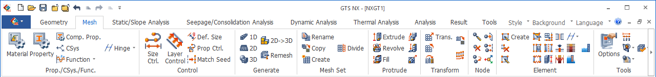
1. Interface
The
interface behavioral model was developed to simulate the
boundary (interface) behavior between same or different
materials. The interface behavioral model is not only
used in geo-technology but also throughout architecture
and civil engineering in general to define the behavior
of various interfaces. The interface behavioral model
is based on Coulomb's
law of friction (1785) and follows the assumption
that the frictional force of an interface is proportional
to the coefficient of friction and the confining forces
perpendicular to the normal direction acting on the interface.
This
model is mostly used to simulate rock joints or structure-ground
interfaces such as friction pile-ground interface, earth
retaining wall-ground interface, lining-ground interface
etc.
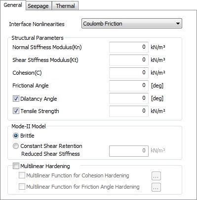
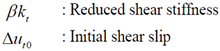
<Coulomb Friction function>
The
main nonlinear parameters of the interface model are as
follows. The user can also define the coefficient of permeability
or stiffness to simulate interface behavior.
[Normal
stiffness modulus (Kn)]
Is
the Elasticity modulus for bonding and un-bonding behavior
in the normal direction to the interface element. The
general range is 10~100 times the smallest value of the
Elasticity modulus on the oedometer of adjacent elements.
[Shear
stiffness modulus (Kt)]
Is
the Elasticity modulus for slip behavior in the normal
direction to the interface element. The general range
is 10~100 times the smallest value of the shear strength
of adjacent elements.
The
nonlinearity of the interface needs to be computed by
applying the Coulomb Friction criterion and using the
stiffness parameters along with experimentation (relative
displacement-frictional force curve), but an empirical
formula can be used to predict the interface behavior
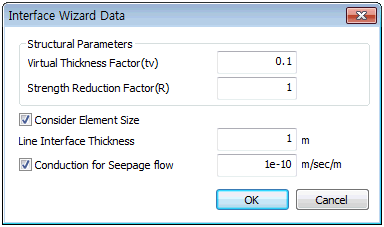
between 2 materials. The empirical formula uses a virtual
thickness (tv) and strength reduction factor (R). When
creating an interface element, the following Wizard can
be used for automatically calculate, according to the
element properties of the neighboring ground element,
using the 2 parameters (tv, R).

The interface material can be defined
using the following equation. Using the stiffness of adjacent
elements and nonlinear parameters, the virtual thickness
(tv) and strength reduction factor (R) is applied. Interface
material stiffness and parameters are applied differently
according to the relative stiffness difference between
neighboring ground and structural members. The Wizard
can be used to simplify this process.
Kn
= Eoed,i / tv
Kt
= Gi/tv
Ci
= R x Csoil
phii = tan-1
(R x tan (phisoil))
Here, Eoed,i
= 2 x Gi x (1-νi)/(1-2 x νi)
(νi
=Interface Poisson’s ration=0.45, the interface is used
to simulate the non-compressive frictional behavior and
automatically calculates using 0.45 to prevent numerical
errors.)
tv
= Virtual thickness(Generally has a value between 0.01~0.1,
the higher the stiffness difference between ground and
structure, the smaller the value)
Gi
= R2 x Gsoil (Gsoil
= E/(2(1+ νsoil)),
R = Strength Reduction Factor
The general Strength reduction
factor for structural members and neighboring ground properties
are as follows.
In
case of multiple soil layer the same structural component,
the smaller value of R is recommended.
Checking the Element size consideration
calculates the interface material properties considering
the average length(line), average area(face) of the neighboring
ground element when creating an interface. In other words,
the average length(l), average area(A) are multiplies
to the virtual thickness in the equation below to calculate
the tangent, normal direction stiffness of the interface.
Kn
= Eoed,i / (I
or √A x tv ) , Kt
= Gi / (I or
√A x tv )
If
the consideration is not checked, the unit length(area)
is applied.
The thickness is defined separately
for a line interface. The thickness is an important element
when using the interface on a ground material that displays
hardening behavior. Generally, the neighboring ground
particle size is input, but if an accurate numerical value
is not available, the default value from the program is
used. For a 3D model, like the 1 in the example above,
the surface interface does not need a thickness.
When defining the stiffness against
seepage for an interface element, the “permeability coefficient”
can be defined to be the same as the permeability coefficient
of the ground. If the option is not checked, the layer
is considered to be impermeable.
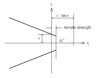
When
the dilatancy angle and tensile strength is defined, a
smaller or equal value needs to be defined for the interface
element and the cohesion; friction angle can be multiplied
with the strength reduction factor. For the interface
dilatancy angle, the same angle can be applied as the
ground when the ground is under rigid body motion without
strength reduction (R=1). When considering strength reduction,
entering '0(zero)' is the general definition for rigid
body motion.
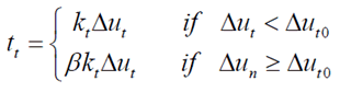
[Mode-II
Model]
The
Mode-II model expresses shear behavior and defines the
tangential slip behavior or the interface. For the 2 models
below, the failure envelopes are shown for when the ‘Constant
Shear Retention’ function is considered suitable in terms
of numerical analysis stability etc.
The structure does not receive
any loading if the vertical force is higher than the tensile
strength.
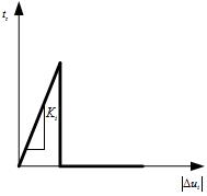
Apply the input value on
the shear direction such that the structure can receive
loading in that direction.
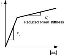
 : Reduced Shear Stiffness : Reduced Shear Stiffness
[Multi-linear
Hardening]
If
a function is entered in the multi-linear hardening, the
cohesion and friction angle used in the Coulomb friction
failure criterion changes with plastic displacement. Note
that the cohesion and friction angle both need to increase
as the plastic displacement increases. This behavioral
characteristic must be defined by experimentation and
is mainly used for research purposes than practical purposes.
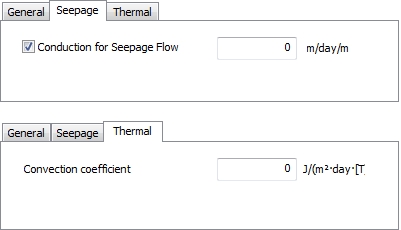
[Conduction
for Seepage flow]
Sets
allowable flow rate at the interface.
[Convection
coefficient]
Controls allowable heat exchange at the interface.
Bond Slip
In
reinforced concrete, the interaction between the reinforcement
and the concrete is governed by secondary transverse and
longitudinal cracks in the vicinity of the reinforcement.
This behaviour can be modelled with a bond-slip mechanism
where the relative slip of the reinforcement and the concrete
is described in a phenomenological sense.
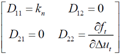
In GTS NX, the relationship
between the normal traction and the normal relative displacement
is assumed to be linear elastic, whereas the relationship
between the shear traction and the slip is assumed as
a nonlinear function.
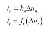
Differentiating
results in expressions for the tangential stiffness coefficients.
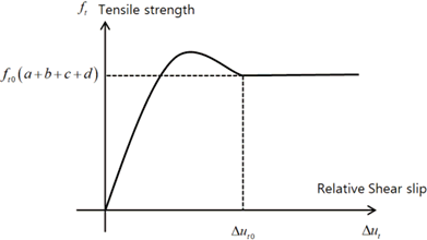
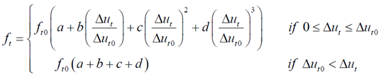
GTS NX offers a predefined curve,
‘polynomial function’, for the relationships between shear
traction and slip, and a user-defined multi-linear function
is also available. The polynomial function describes the
relationship between shear stress and slip as shown in
the figure below, and the formula is shown below.
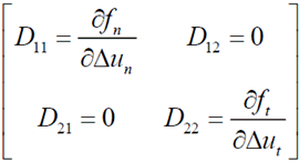
Discreet Cracking
The constitutive
law for discrete cracking in GTS NX is based on a total
deformation theory, which expresses the tractions as a
function of the total relative displacements. The relationship
between normal traction and crack width and the relationship
between shear traction and slip are assumed as nonlinear
functions.
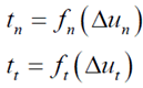
In the above equation, the relationship
between the normal traction and shear traction is independent
to each other, so the stiffness can be expressed as follows.
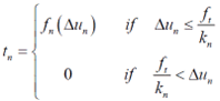
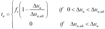
In general, the normal traction is
governed by a tension softening relation. For structural
interface elements, GTS NX supports the following relations:
Brittle Cracking Model -
Brittle
cracking model is characterized by the full reduction
of the strength after the strength criterion has been
reached.
Linear
Tension Softening Model
In
case of linear tension softening, the relation of
the crack stress and displacement in the normal direction
is given by the figure below.
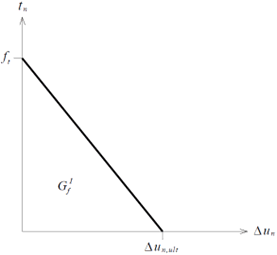
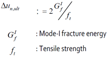
Unloading and reloading
can be modeled according to a secant approach or an elastic
approach. In the secant approach, the relation between
the traction and the relative normal displacement is linear
up to the origin, after which the initial stiffness is
recovered. In the elastic approach, the initial stiffness
is recovered immediately after the relative normal displacement
has become less than the current maximum relative normal
displacement.
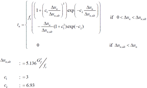
Non-Linear Tension
Softening Model
Hordijk , Cornelissen
& Reinhardt proposed an expression for the softening
behavior of concrete as shown in the figure below.
Unloading
and reloading can be modeled according to a secant approach,
an elastic approach or by application of hysteresis.
Shear Retention
In general, the shear traction is
reduced after cracking according to the following equation
In general, β may vary between
0.1 and 0.3. If the crack surface is assumed to be smooth
after Mode-I cracking, β is defined as zero. But
generally, it is assumed that the crack surface is not
smooth and β and hence 0<β<1.
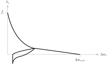
2.Shell Interface
The
interface element was developed to simulate the interface
behavior just like a general face element. Here, the interface
element is also capable of resisting the rotational force
between plates.
Tensile
force is not transmitted to the load or moment. Linear
behavior is observed for small rotations or shear
force. Nonlinear
elastic behavior for large rotations. (Janssen’s law) Plastic
behavior for large shear force. (Coulomb friction)
Nonlinear
behavior at the plate interface element follows the Coulomb
friction law for movement and Janssen’s law for rotation.
The relative move displacement and interface force follows
the Coulomb friction model with some restrictions. The
tensile strength is set as 0 for the Tension Cut-off function,
the dilatancy angle and interior friction angle are identical
and the asymmetrical material property matrix is not defined.
The stiffening function does not need to be defined separately.
For
the User supplied shell interface, it is the same as the
"User
Suplied Material" model.
Janssen's Law
The Janssen model, which is
applied to the rotational DOF of shell interface elements,
simulates the nonlinear elastic relationship between the
moment and rotational displacement. GTS NX provides for
the Coulomb friction model and Janssen model for shell
interface elements. The Coulomb friction model is used
to define the normal and lateral direction forces.
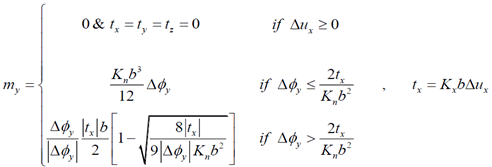
Only perfectly plastic
behavior is supported for Coulomb friction models used
on shell interface elements.
|