The figure above is the Analysis control and Result control setting windows. The additional setting control options for each analysis type is shown, and the detailed inputs are listed in the table below.

    ( * : Time step setting analysis type )

<Table.Static analysis - Analysis control options for each analysis type>

    (* : Time step setting analysis type )

<Table. Dynamic analysis- Analysis control options for each analysis type>

<Table. Thermal analysis- Analysis control options for each analysis type>

Water Pressure (Automatically consider water pressure)

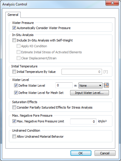
Analysis Control dialog windows for Linear Static and Construction Stage analysis types

This option considers all free surfaces/edges of the model as an external water pressure. The water pressure is calculated with reference to the pore pressure acting on the free surface/edge.

• If water level is set, assume constant water pressure with reference to the water pressure.

• If seepage analysis was conducted previously, use the pore water distribution (size) calculated for each node.

• If the pore pressure is a negative (-) value, water pressure is not considered automatically

Caution: If modeling is done for the case where the external water pressure corresponding to pore water pressure in the model does not exist, this option needs to be canceled. When conducting stress analysis by specifying the water level line, the pore pressure is calculated by the water level difference between the free node and corresponding load. Hence, to accurately examine the influence lines of the underground water level, Seepage-stress coupled analysis is recommended.

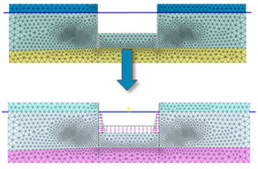
<Application of auto-water pressure on excavation surface when excavating below the water level>

In-situ analysis

[Include in-situ Analysis with Self-weight]

This option resets the stress state of the singular analysis ground. The calculated in-situ stress is in equilibrium with the self-weight and the same boundary conditions used in singular analysis for analysis. When considering self-weight in time history analysis, the initial in-situ stress needs to be calculated. If not, vibrations can occur due to the load addition. In particular, the self-load must be included for nonlinear time history analysis.

[Ko condition consideration]

The  method uses the constant defined by to calculated the horizontal stress from the vertical stress to set it as the in-situ stress.

Using this method, the vertical stress needs to be found first using self-weight analysis and that value can be used to compute the horizontal stress using . Here, the shear stress maintains its value, calculated from the analysis result.

If the ground surface is horizontal, there are no problems in using this method, but if not, the calculated stress state and self-weight are not in equilibrium.

If the stress is adjusted without maintaining the equilibrium state, the stress can change to fit the equilibrium with the external force in future stress analysis, even if there are no external force changes, causing deformation. Hence, the  method can be applied if the additional stress changes are relatively small. Generally, the conditions when the stress modification due to the method can be used are as follows.

• When the ground shape change in the horizontal direction is small

• When the pore pressure distribution shows no change in the horizontal direction

• When the horizontal stress can occur due to the horizontal boundary condition of the free line/face

• When using transversely isotropic materials that have the same material vertical/horizontal axis

If the condition is not considered, the stress state obtained from the self-weight analysis is set as the in-situ stress. If the ground surface is horizontal, this method is the same as the method when . If not, a horizontal strain exists and different results than the method results can be obtained. Shear stress also occurs.

This method is generally recommended when the ground is sloped. However, because a value larger than 1 cannot be set for the value, a null stage can be added for re-analysis after using the method to calculate the equilibrium stage, without adding extra external conditions when a value larger than 1 is needed. However in this case, the final equilibrium state does not satisfy the condition. Also, the modified stress is vastly different from the equilibrium point, it can be hard to calculated a converging solution using nonlinearity.  

Initial Stress

[Estimate Initial Stress of Activated Elements]

In order to calculate the initial stress of ground, FEA NX perform Linear Analysis even if nonlinear material is assigned to the elements. In this case, it can result in, sometimes, over-estimating the soil behavior  (large displacement). Initial Stress Options can eliminate this problem especially for newly activated elements which are to simulate a fill-up ground such as backfill and embankment.

[Engineering example]

[Clear Displacement/Strain]

The displacement reset condition may be needed during analysis. For example, when the displacement and strain due to self-weight need not be considered in the initial analysis stage, the reset option can be used to reset the in-situ state displacement and strain to ‘0(zero)’.

Also, the reset can be performed at an arbitrary construction stage, such that the middle stage after analysis of several stages can be set as the reference state. Displacement/Strain reset is applied at the end of the specified stage, after the analysis has finished.

Caution: When conducting nonlinear analysis by considering geometry nonlinearity, arbitrarily modifying the deformation does not guarantee the continuity. Hence, this option is not recommended for geometric nonlinear analysis of construction stages.

[Cut-Off Negative Effective Pressure]

When conducting linear static analysis for initial stress of ground, tensile stress can be generated especially at the ground surface according to the geometry and stiffness differences. In this case, this tensile stress can take effect on the convergence for the following stage (nonlinear analysis) significantly.  If there is tensile stress generated in in-situ state, software will make it close to Zero to ignore the abnormal stress distribution. Since this is the basic concept of initial stress of ground, strongly recommended to use for all staged analysis.

Initial Temperature

This option sets the initial temperature of the single analysis model. If not checked, the initial temperature defined in the [Analysis Control] is considered. The temperature is used to assess the effects of thermal load, and the temperature difference with the input temperature load is considered in the analysis.

Water Level

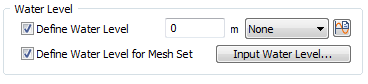
[Define water level]

Directly input the water level height, or select a water level function that already has a specified water level to set the water level. The set water level is applied to the total model. When using the water level function, the input value is multiplied to the function value and applied.

[Define water level for mesh set]

Define the water level for each mesh set.

If the groundwater layer is surrounded by rocks or an impermeable clay layer (confined aquifer), the presence/absence of the groundwater level for each ground layer can be set for analysis.

If the total groundwater level is input and a mesh set has a defined groundwater level, the mesh set groundwater level has priority and the total groundwater level is applied to mesh sets that do not have a defined level.

If the water level and the function are specified at the same time, the input water level and the function are multiplied and reflected in the analysis.

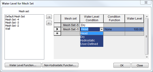
Mesh Set – select the mesh set to apply the water level condition.

Water Level Condition – select between Head, Dry, Hydrostatic and User-Defined for applying water pressure

   Head – compute head according to the water level assigned to the mesh set.

   Dry – assume there is no pore water pressure applied to the mesh set.

   Hydrostatic – assign a non-hydrostatic water pressure to a mesh set.

   User-Defined – apply a user-defined pressure gradient to a mesh set

Condition Function – select a condition function for Head, Hydrostatic & User-Defined

• Head  

            -     None – set a single water level for water pressure calculation.

            -     Water Level Function – assign a function which describes the water level using General Function in 2D  and Surface Function in 3D. 

• Hydrostatic – not available

           -  Water Level Function – assign a Non-Hydrostatic Water Pressure function type Hydrostatic to define a pressure profile to be used to compute the water pressure.

•  User Defined

          -  Water Level Function – assign a Non-Hydrostatic Water Pressure function type User-Defined to apply a linear pressure profile.

Water Level – input water level to be considered for the selected mesh set (only for Head).

Saturation Effects

This option is to conduct accurate analysis when the saturation has a value between the unsaturated state (Se=0) and the saturated state (Se=1). The partial saturation can be applied in the following two cases.  

• Applying the partial saturation to calculated the effective stress-total stress relationship (Use Bishop’s effective stress relationship equation)

• Consider the partially saturated state in the unit weight calculations for a material, such that the unit weight when partially saturated has a value between the saturated unit weight and unsaturated unit weight.

If partial saturation is not considered, Terzaghi’s effective stress formula is used and the unit weight is set as either the saturated unit weight or the unsaturated unit weight, depending on the pore water pressure distribution (a value in between is not used.). The saturation is defined as a function of pore water pressure and if partial saturation is considered, the unsaturated properties of the material need to be defined to define the saturation function for pore water pressure.  

Maximum negative pore water pressure limit

This option limits the maximum negative pore pressure by the input number. If partial saturation is not considered, Terzaghi’s effective stress formula is used and the pore stress of the unsaturated state can be overly reflected in the calculation. Hence, when not considering partial saturation, the negative pore water pressure needs to be limited to a certain value. Reversely, if the partial saturation is considered, Bishop’s equation is used and there is no such danger. In other words, the pore stress is limited by the unsaturated property function and there is no need for a particular limit on the negative pore water pressure.

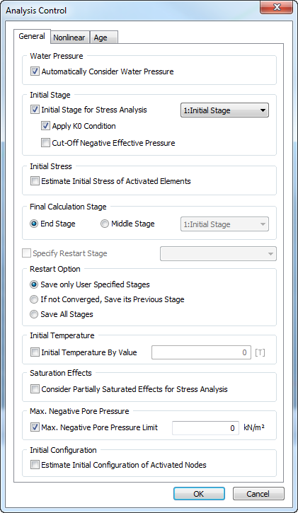
Construction stage general setting

[Initial stage]

Specify the construction stage that will be considered as the in-situ condition and check the Ko consideration. Refer to the ‘Linear analysis’ option for more information on the Ko. The displacement and strain for the construction stage specified as the initial stage, is reset.

[Initial Stress]

In order to calculate the initial stress of ground, FEANX perform Linear Analysis even if nonlinear material is assigned to the elements. In this case, it can result in, sometimes, over-estimating the soil behavior  (large displacement). Initial Stress Options can eliminate this problem especially for newly activated elements which are to simulate a fill-up ground such as backfill and embankment.

[Final calculation stage]

The default setting is calculation up to the final stage, but a separate Final calculation stage can be set when stopping the analysis to check the interim results.

[Specify restart stage]

When specifying the construction stage, the [Specify restart stage] option can be checked on the Analysis control for each stage. The checked stage is automatically saved on a separate result file and when the same model is used for re-analysis, the re-analysis can be performed starting from the next stage of the result file. It is useful when many construction stages are specified.

[Restart option]

If the converge standard is not satisfied for non-linear analysis, the reliability can be in question and so, it is important to check whether the converge standard is satisfied for each stage during construction stage analysis. In particular, because construction stage analysis can take longer time than single analysis, the [If not converged, save its previous stage] option is available when a stage does not satisfy the standard. This option saves the stage before as a result file and the model can be review and modified before restarting. Also, the [Save all stages] option is available for when the analysis is terminated forcefully, due to the computer system instability or to check the interim results. However, because saving all analysis results takes up a large size, the save capacity needs to be secured on the computer.  

Initial Configuration

During construction, the newly activated nodes(elements) can be set to the position considering deformed shape in the previous stage. Following is the example of staged embankment to compare the settlement distribution between with and without applying the option.

[With option vs Without option]

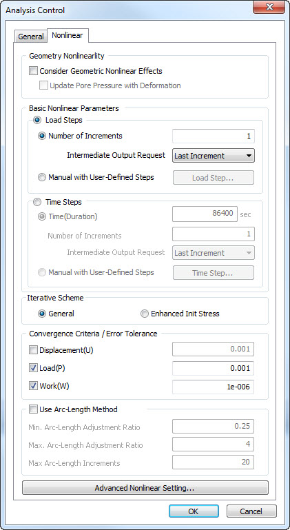
Geometry Nonlinearity

In case of large deformation analysis, the user can check more reasonable behavior with this option. This is to consider geometric nonlinear effects in stress, fully coupled and slope stability analysis. Analysis can take into account load nonlinearity which is reflecting the effects of follower loads, where the load direction changes with the deformation. Depending on the deformed shape, the pore water pressure can be updated automatically.

Load steps (or Time Steps)

A static load can be used for nonlinear static analysis. The defined load sum can be applied at once or in stages, as an increment, cumulatively. If the load increment is too large, it may be hard to calculate the converging solution and if the load increment is too small, unnecessary is spent on calculations. In case of considering time-dependent material, the user can define Time steps to check the results with time elapse.

Convergence Criteria

Because nonlinear analysis uses iteration methods, the converge condition can be used to determine whether the solution has converged. The convergence is determined by comparing the displacement, member force or energy change in the previous calculation with the reference values. If all selected conditions are satisfied, the iteration is determined to have converged.

Use Arc-Length Method

FEA NX uses the Newton-Raphson method, where the increments are calculated to minimize the error repeatedly, as a base for calculating the nonlinear analysis solution. The Full Newton-Raphson, which renews the stiffness matrix for each repeated calculation, is basically used and the Newton-Raphson method or Initial stiffness method can be used at the renewal point. Also, other various options such as the line search method to improve the convergence, or arc length method, to calculate the unstable equilibrium state, can be used (Refer to Chp.5-5 of the Analysis manual for more details). The iterated calculation method repeats the calculation until a satisfactory solution is obtained. If there is no accurate numerical basis, the initial setting value is recommended.

[Minimum arc-length adjustment ratio]

Input the minimum change to the initial arc length to current increment arc length ratio. This prevents the arc length from becoming infinitely small.

[Maximum arc-length adjustment ratio]

Input the maximum change to the initial arc length to current increment arc length ratio. This prevents the arc length from becoming infinitely large.

[Maximum arc-length increments]

Input the maximum number of increments. Nonlinear analysis using the explicit arc length method is conducted until the load factor is larger than 1, or when the number of increments reaches the maximum value. The explicit arc length method may not work, according to the load in the problem, and the number of  maximum allowable load increments is input to prepare for this.

Advanced nonlinear setting

The basic settings use the nonlinear analysis parameters and the [Use default settings] option is selected for most problems. The detailed settings are as follows.

[Stiffness update scheme parameter]

The Full Newton-Raphson, which renews the stiffness matrix for each repeated calculation, and the Initial stiffness method, which maintains the initial stiffness matrix and has very weak nonlinearity, are available. Other options such as the Modified Newton-Raphson method or Secant method, which increases the convergence and efficiency of the Newton-Raphson material properties, can be selected. Refer to Chp.5 of the Analysis manual for more details on the algorithms. The user can also specify a method to recompose the stiffness matrix by selecting repetition, semiautomatic and automatic.

[Analysis option]

• Terminate Analysis on Failed Convergence : Close analysis when convergence fails. If the option is not selected, the analysis is continuously conducted even when the values to not converge.

• Max number of Iterations per Increment : Input the maximum number of iterations for one increment. [Maximum Bisection level] : Specify the maximum division level.

• Enable Line Search : Use the line search feature. This feature is helpful for problems with flexible structures, where the stiffness increases with the load, or if the nonlinear analysis solution converges while vibrating. It may only increase the analysis time when used on an ineffective problem.

• Max Line Search per Iteration : Input the maximum number of line search per repeated calculation.

• Line Search Tolerance : Input the line search tolerance.

• Divergence Threshold : Specify the number of allowable diversions if the value does not converge. The modified Newton-Raphson method renews the stiffness matrix at the start of each load increment.

Age

In case of construction stage analysis, the user can take Age into account to consider creep / shrinkage effect generated in the previous stage. For the time-dependent material, the user, in general, can enter the curing period of concrete.

Initial condition (Seepage)

This option specifies the initial pore water pressure distribution in the ground for transient seepage analysis. The initial conditions must be set for the transient analysis. The initial condition can be selected by using the  values at time ‘0(zero)’ of the transient time step, using an arbitrarily set water level height, or using the water level function.

Safety factor (SRM)

Input the initial safety factor and the safety factor increment for each repeated calculation step. The resolution of safety factor can also be set.

[Resolution of Safety Factor] - Slope analysis using SRM uses the strength reduction method, and the resolution of safety factor value can be input to specify the accuracy of the safety factor calculation. The resolution of safety factor is used as a convergence standard for stability analysis. However, if the resolution of safety factor is entered too low, the analysis time increases greatly and so, the following guideline needs to be used to input an appropriate value.

<Table. Dynamic analysis- Analysis control options for each analysis type>

Eigenvectors

Input the number of natural frequency modes (number of modes) to input and specify the range to search. The option to check for any omitted eigenvalues can be applied.

Mass parameters

[Coupled Mass Calculation]: Use a mass matrix that considers the coupling between modes. Check to use a consistent mass matrix, and uncheck to use a lumped mass matrix. It is hard to determine which is more accurate, but for eigenvalue analysis, using a lumped mass matrix displays a more flexible behavior than using a consistent mass matrix.

Modal Damping Ratio

Calculate Strain Energy Proportional Damping Ratio

Eigenvalue analysis provides damping ratios for each mode based on the strain energy of the structure. This can be used to obtain modal damping ratios in the structure with different materials or damping devices. The modal damping ratio can be found after analysis from Result > Advanced > Others > Modal Damping Ratio.  

Modal combination type

If the maximum actual physical quantity is assumed to be the maximum physical quantities (maximum values for displacement, stress, member force, reaction force etc.) of each mode, the maximum values of each mode can simply be added. But because there is no guarantee that the maximum values of each mode occur on the same time step, it is difficult to express the maximum actual physical quantity through simple linear super positioning.

Hence, a mode combination method to approximate the maximum value is needed. Various mode methods are suggested, but because no one combination can give the appropriate approximation for all cases, the characteristics of each mode combination needs to be understood. The modal combination types are as follows, and refer to Ch.5 of the Analysis manual for more detailed algorithms.

• ABS(summation of the Absolute value)

This method assumes that all mode responses occur on the same phase and the maximum value for each mode is judged to occur on the same time step, giving the most conservative results.

• SRSS(Square Root of the Summation of the Squares)

This method provides appropriate results when each mode is sufficiently separated.

• NRL(Naval Research Laboratory method)

This method removes one mode( ) that has the maximum absolute value from the SRSS method, and like the SRSS method, this method provides appropriate results when each mode is sufficiently separated.

• TENP(TEN Percent method)

This method includes effect of adjacent frequency modes in the SRSS. In other words, if two mode frequencies satisfy the following, the two modes are determined to be adjacent, within 10% of the frequency.

• CQC(Complete Quadratic Combination method)

If the cross-correlation coefficient between modes is 1, it displays the same results as the SRSS method.

Damping definition

[Direct modal]

The user directly defines the damping ratio of each mode, and the mode response is calculated using that ratio. The direct modal method is only activated for Response spectrum / Time history (Modal) analysis.

• Damping Ratio for All Modes

Define the default damping ratio that is applied to all modes, except for the ones defined by the user. The default damping ratio is applied to all modes that have a lower priority than the specified mode. If the input damping ratio is different from the damping ratio of the response spectrum function, the spectrum data is adjusted with reference to the input damping ratio and used for analysis.

• Modal Damping Overrides

It is used to directly input the damping ratio for each mode. The mode number and mode damping ratio are input separately and then added.

[Mass Stiffness Proportional]

Compute the damping constant for mass proportional attenuation and stiffness proportional attenuation. The proportional coefficient can be directly input, or automatically calculated from the mode attenuation, for checked items on the attenuation type.

Input the mode frequency or period and specify the damping ratio to automatically calculate the proportionality coefficient.

Here, the attenuation for each material, when calculating the mass & stiffness coefficients from the modal damping, can be reflected in the analysis. The damping ratio of each material, input in the [Show Coefficients from Material], and the damping coefficient (alpha, beta) of the damping matrix, calculated using that value, can be checked.

Interpolation of Spectral Ratio

Select the interpolation method for the response spectrum load data. Both linear interpolation or logarithmic interpolation can be used for the spectrum data period and the default setting is the logarithmic interpolation method. If multiple damping ratios are in the spectrum data, interpolation of the damping ratio also follows this option. Spectrum data with one damping ratio cannot be interpolated and is corrected using the following equation. (1.5/(40xAttenuation+1) + 0.5)

Define Time (Nonlinear time history + SRM)

Specify the time to view the SRM analysis results. Multiple time steps can be specified. The SRM stability assessment is conducted using the nonlinear time history stress results from the specified time period.

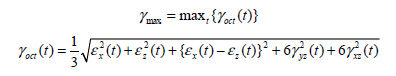
Effective shear strain (2D equivalent linear analysis)

The shear strain of the ground changes with the input seismic motion or vibration load. To apply equivalent linear analysis, the concept of effective shear strain is introduced, and the material properties are simplified to have equivalent linear values for calculation.

Frequency domain analysis is analyzed to have a certain shear modulus and damping for each frequency, and the material nonlinearity cannot be considered. Hence, the 2D equivalent linear analysis uses iterated calculations, using the changing ground stiffness and damping ratio due to the shear strain calculated in the previous stage, to consider the nonlinear behavior of the ground. Here, the maximum shear strain used in the previous stage is multiplied by a certain value(50%~70%) smaller than 1 to define the effective shear strain. The effective shear strain is used because the maximum shear strain generates a larger strain energy than the actual  behavior.

Generally, an effective shear strain coefficient of 0.65 (65%), or the value that uses the earthquake magnitude is used. Also, a maximum shear strain calculation method in the time domain is supported to calculate shear strain more precisely than the maximum shear strain found using the RMS(root mean square) in the frequency domain.

<Difference between maximum and effective strain>

There are two methods to calculating the maximum shear strain; the time domain and frequency domain. The time domain method defines the load (acceleration, force etc.) changes according to time and composes the structural state as a differential equation. Hence, the structural response (displacement, velocity, acceleration response) can be calculated by performing the integration for every time interval. The frequency domain method is useful when determining the relationship and ratio between the load response and frequency characteristics. Because it is hard to determine this relationship and ratio for irregular waves such as earthquake response, the wave in the time domain is converted to the frequency domain and used for analysis.

[Interpolation control]

Input the frequency range for frequency domain analysis. Interpolation methods are used to efficient frequency domain analysis and one of the four methods can be selected.

Select [Coupled Mass Calculation] to conduct the analysis for all frequencies and if the interval is specified, the analysis frequency interval in the frequency domain becomes the set interval.