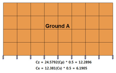
Approximately express the semi-infinite ground layer by setting a virtual slip surface perpendicular to the horizontally layered ground. This is done to consider the surface wave propagation into the far-field ground.

The transmit boundary condition is only used for Dynamic analysis > 2D Equivalent linear analysis.

The boundary conditions in ground modeling can be largely divided into:

1.  [Element Boundary Condition]

2.  [Viscous Boundary Condition]

3.  [Transmitting Boundary Condition].

1. The [Element Boundary Condition] can be divided into: 1) the free end, where the force of the earthquake response load is input, and 2) the fixed end, where the displacement is input at the free field boundary position. The [Element Boundary Condition] can consider the effects of earthquake waves in the free field, but it does not consider the effects of waves reflecting off the foundation slabs of an existing structure. This effect gets larger as the boundary position moves closer to the foundation slab.

2. The [Viscous Boundary Condition] was developed as a solution to the flaws of the [Element Boundary Condition] using a boundary condition that absorbs material waves having a certain angle to the boundary, developed by Lysmer & Kuhlemeyer, Ang & Newmark, etc. However, because the [Viscous Boundary Condition] cannot fully process the effects of complex surface waves, the boundary needs to be set at a certain distance from the foundation slab, as with the element boundary.

3. The [Transmitting Boundary Condition] supplements the flaws of the [Viscous Boundary Condition] and considers the effects of nearly all types of material and surface waves. The horizontal soil layer can be expressed as a spring and damper using a function of frequency. 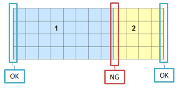The [Transmitting Boundary Condition] generally assumes that the horizontal properties of each ground layer are equal and so, satisfactory results can be obtained even when the boundary condition exists at the structure itself. However, to accurately consider the property changes due to horizontal deformation, it is effective to maintain a certain distance between the boundary and foundation slab.

General

Select the element edge and line to set the transmit boundary on that element edge. The ground information assigned to the element can be used to create the transmit boundary.

When the line between 2 different elements is selected, the transmit boundary is not created.

Auto

Selecting a mesh set automatically creates boundary conditions and elements at the left/right/floor of the mesh, according to the user specified options. The spring constant value is calculated depending on the ground material characteristics defined for the mesh set.

The right/left transmit boundaries of the analysis model can be set, and the viscous boundary can be created at the floor surface and free face.

It is difficult to accurately simulate the ground, which exists almost infinitely, using a 2D model used in Ground-Structure Analysis. Hence, the model boundary needs to be set at an engineering-appropriate position and processed to simulate in-situ conditions.

Boundary Set

Register the set constraint conditions on the desired boundary set. The user can specify the name of the boundary set.

Auto create viscous boundary

The Viscous boundary condition can be created as follows.

1. Compute Cp and Cs

The Cp and Cs are calculated using the equations below:

Here, ,  

λ : Volume modulus, G : Shear modulus, E : Elastic modulus, ν = Poisson’s ratio,

A : Cross-section area

• Multiplying the Cp, Cs (tonf•sec/m^3 units) by the cross-section area eventually leads to the spring stiffness of the viscous boundary element in tonf•sec/m units.

• The shaded cell parameters are the physical properties of the ground that the user inputs during modeling. The volume modulus and Shear modulus are calculated using the Elastic modulus and Poisson’s ratio. Hence, there is no need to input additional values when creating a viscous boundary element.

• When creating the bottom viscous boundary element, the spring is automatically created by considering the element area (effective length*unit width) as shown below.

• Input the Cp value for the normal direction coefficient at the point of spring creation and input the Cs value for the parallel direction. Hence, the bottom spring coefficient Cz becomes the Cp value and the Cs value is applied to the Cx.

<Auto-create viscous boundary>