|
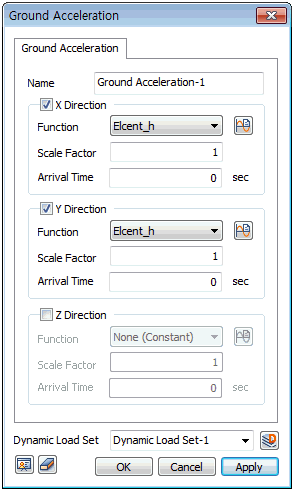
[Direction]
Define the input (transmission) direction of ground acceleration. It is set with reference to the global coordinate system (GCS) and multiple directions (X,Y,Z) can be combined to set a single ground acceleration load set. The increment coefficient for the ground acceleration can be defined using a scale factor and the arrival time can be controlled to set the ground acceleration delay time.
[Function]
Select the  button to define the ground acceleration function. button to define the ground acceleration function.
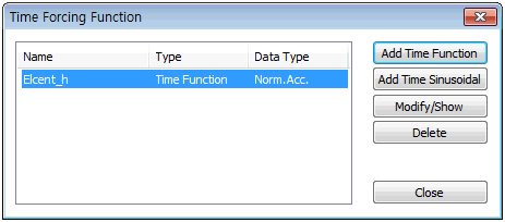
Add time function
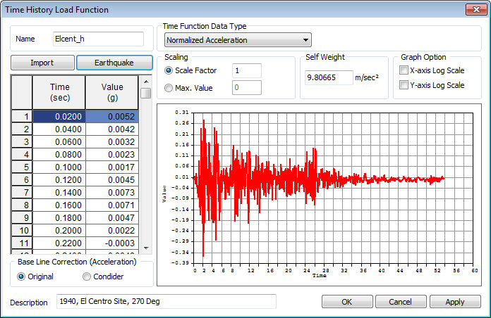
Construct the time varying load by directly entering the time and the corresponding time varying load value in the left input column on the dialog box. The time function data types are classified by Acceleration, Force(load), Moments, Normalized Acceleration (Time history acceleration / Gravitational acceleration) or Normal(generalized). Changing the data format only changes the application format, not the data format. The scale factor is a gradient modulus for the entered data. The entire data can be scaled to fit the specified maximum value.

Time function load application
The defined function is also applicable for [Dynamic nodal (surface)] and [Time varying static]. Specifying 'force' or 'moments' uses the time varying load as a [Dynamic Nodal(surface)] input and specifying 'Normalized acceleration' or 'Acceleration' uses it to input the [Ground Acceleration]. Specifying ‘Normal’ uses the time varying load as the change in static load with time for [Time Varying Static] or [Dynamic surface].
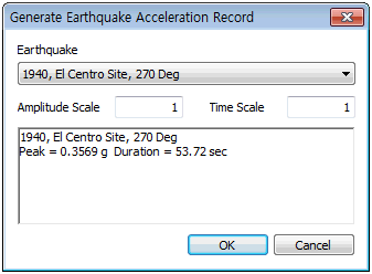
Import/Earthquake waves
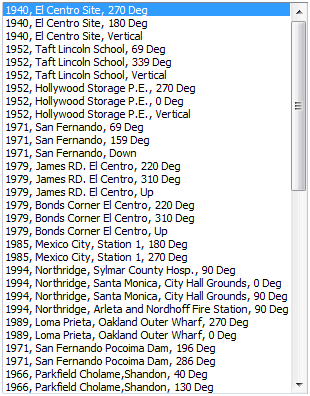
Save and import frequently used time varying load or select earthquake acceleration data from the program DB. There are a total of 32 types of earthquake accelerations.

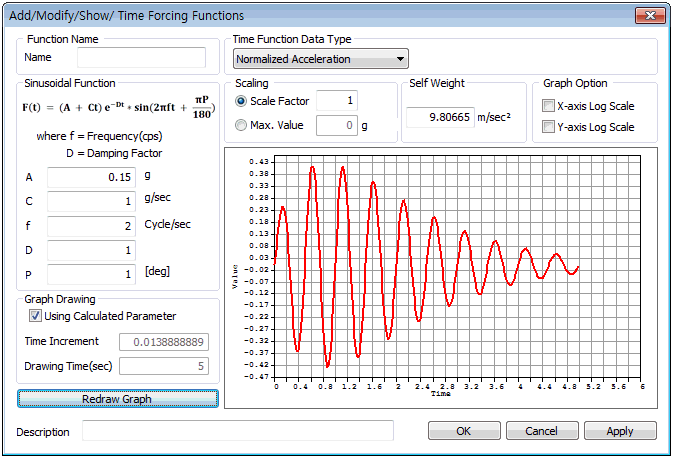
Add Time sinusoidal
A sine function can be used to define the time varying load. A and C are constants, f is the frequency of the input load, D is the damping factor and P is the phase angle. If the time varying load is entered as a harmonic function, input the necessary sine function variables and click [Redraw Graph] to view the loading on the right hand side.
|