|
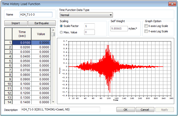
Select the static load to be applied on the load set. The load application position, direction and size are already determined when entering the static load, and the to-be applied time forcing function is selected. The gradient modulus of the load can be defined by a scale factor and the arrival time can be set to simulate the delay time.
Select the  button to add (select) a time forcing function. It can only be applied when the time forcing function data type is ‘Normal’ (dimensionless function) button to add (select) a time forcing function. It can only be applied when the time forcing function data type is ‘Normal’ (dimensionless function)

Construct the time varying load by directly entering the time and the corresponding load change ratio in the left input column on the dialog box. The scale factor is a gradient modulus for the entered data. The entire data can be scaled to fit the specified maximum value.
|
