General function(Spatial)

Changes in position (coordinates) of a value with respect to the rectangular or cylindrical coordinate system can be set as function and used when specifying the load. The water level conditions can be directly specified on the screen, but registering the water level according to the coordinate change as a function allows this to be used as the water line during the construction step.

Input the independent variables (X,Y,Z or R,TH,Z) according to the reference coordinates and the values of the set variables in the table to generate a function . Already made functions can be copy + pasted from Excel.

<Reference coordinate system standard>

[Equation]

The Equation can be set without defining the values of the independent variables.

For example, when defining the function Y=2*X on the Cartesian coordinate system, specify the X coordinate range (start, end) and the X coordinate increment first. Input 2*X and press the calculate button to automatically generate a function as shown above.

When defining the function Sin(T) between a certain angle with reference to the T coordinate on the cylindrical coordinate system , specify the angle range (start, end) and increment angle and then input sin(T) to generate a sin function within the specified angle range.

[Scale Value]

Value multiplied to the defined function value. The initial value is set as 1. For example, to increase all defined functions by 2 times, input 2 for the scale value.

[Extrapolation]

Assign a function value to values outside the independent variable range. The user can select whether to set the function value outside the range to be 0, the same as the closest function value or determined through linear extrapolation.

<Extrapolation>

General function (Non-spatial)

Used to specify the shear stiffness and spring stiffness of pile or pile tip elements as a function. The relative displacement vs Force/Area is used as a shear stiffness function and the relative displacement vs Force/Length is used as a spring stiffness function at the pile tips. Different pile shear stiffness functions can be set for each depth when defining the pile material properties.

Generalized space function

The purpose and functions are the same as the general function (spatial). However, the generalized space function is able to generate a function that considers all 3 axis directions while the general function (spatial) is a 1 dimensional function that can only set 1 independent variable axis. The input method and detailed functions are the same as the general function (spatial).

Input the independent variables (X,Y,Z or R,TH,Z) according to the reference coordinates and the values of the set variables in the table to generate a function . Already made functions can be copy + pasted from Excel.

Surface function

Used to specify the water level surface in 3D space. The 3D water level surface can be generated by entering the variable values with reference to the global or cylindrical coordinates as shown in the table below, but it can also be generated using the Boundary Condition > Water Level operation and selecting a surface in space to automatically extract the coordinate information. Here, the X axis spacing determines the precision of the water surface and for suddenly changing sections, the spacing needs to be carefully set following the element node positions.

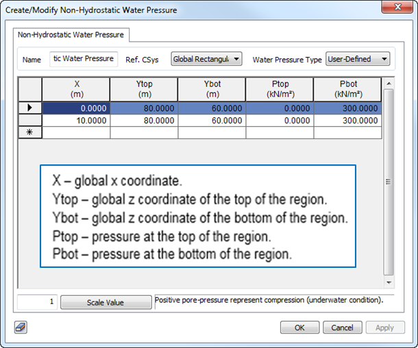
Non-Hydrostatic Water Pressure

Define the water pressure at the top and bottom depending on the position of the model.

 Applicable in integer conditions and user-defined conditions when specifying the mesh set level.

 - User-defined condition: the user can directly define the water pressure at the top and bottom of the assigned mesh by using the specific water pressure function

- Hydrostatic condition: this function is used to define the water pressure at the top of the allocated mesh as hydrostatic.

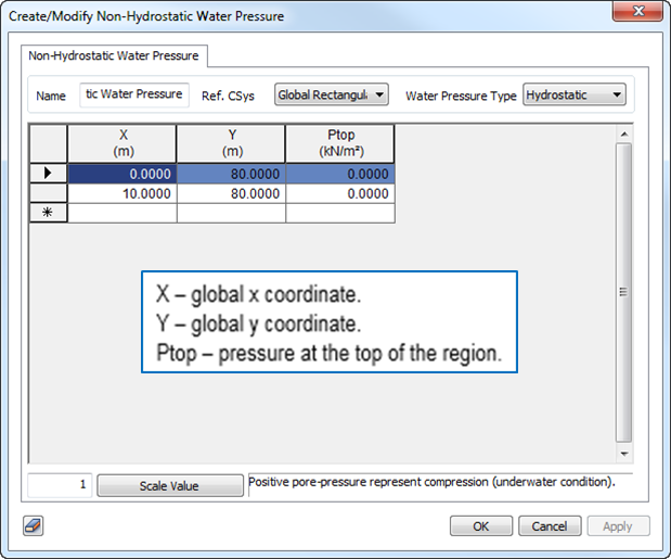
Name – input name for the function.

Ref. CSys – reference coordinate system for the function definition.

Water Pressure Type – select the type of function for selection in Analysis Case > Analysis Control > Define Water Level for Mesh Set. (User Defined or Hydrostatic condition)

Scale factor to multiply all input data.

Creep / Shrinkage Strain Function

Define the time dependent creep property and shrinkage strain of concrete material. These functions are available if User Defined is selected in the Code field.

There are three types of Creep function data types.

 Specific Creep ; Strain per unit stress excluding immediate deformation

 Creep Function ; Strain per unit stress including immediate deformation

 Creep Coefficient ; Ratio of creep strain to elastic strain

A frequently used Creep Function may be saved in and recalled from a file. The data file, fn.TDM retains the following form:

Creep / Shrinkage Function Group

The user can define Creep/Shrinkage Function based on the embedded Design Codes as follows.

Link to Creep / Shrinkage Design Code

Elastic Modulus Function

Define Time-dependent Elastic modulus function based on selected design code. It is required to input End Time of function with the number of steps.

Link to Elastic Modulus Design Code

Plastic Hardening Function

Shear Hardening in Modified Mohr-Coulomb model can be defined by Equivalent plastic strain related to the mobilized shear resistance. Using "Auto-Calculated" option, solver recalculates friction angle based on the deviatoric plastic strain.

Hardening Curve

Plastic strain and stress are directly inputted. It is used when defining hardening curve within von Mises model. Plastic strain begin once the material starts yielding so it can be calculated using following equation.

Stress-Strain Curve

Stress and stain are directly inputted. It is used when defining Stress-Strain Curve within von Mises model. When Load-Displacement Curve is already known, true strain can be calculated using following equation.

Cohesion Hardening Curve

Plastic strain and cohesion are directly inputted. It is used when describing Cohesion Hardening Curve within CWFS(Cohesion Weakening and Frictional Strengthening).

Frictional Angle Hardening Curve

Plastic strain and frictional angle are directly inputted. It is used when describing Frictional Hardening Curve within CWFS(Cohesion Weakening and Frictional Strengthening).

Dilatancy Angle Hardening Curve

Plastic strain and dilatancy angle are directly inputted. It is used when describing Dilatancy Hardening Curve within CWFS(Cohesion Weakening and Frictional Strengthening).

Tensile Strength Hardening Curve

Plastic strain and tensile strength are directly inputted. It is used when describing Tensile Strength Hardening Curve within CWFS(Cohesion Weakening and Frictional Strengthening).

Seepage Boundary function

Used to simulate the head and flow rate difference with time such as node head, node flux rate, surface flux. Setting the values (head/flux) according to the time flow that fits the specified time unit generates a function that can be applied to unsteady infiltration analysis.

For unsteady infiltration analysis, the time steps for result verification are set separately and the time function for the steps is used in the analysis. When the time step is beyond the range of the function, the function value is automatically calculated using linear interpolation. In other words, to apply a 0 function value to time steps outside the range, the same function value (0) needs to be entered for arbitrary time steps when creating the function as shown in the figure above.

Nonlinear elastic function (Truss element)

The behavioral characteristics of truss elements or embedded truss elements can be defined as nonlinear elastic. The stress change according to strain of the truss element can be directly generated as a function and used. The function can be applied to the tensile (compression) test results of a structural member (truss affiliated) or to the deformation behavior properties of a general steel member.

Nonlinear elastic function (Point spring/ Elastic link)

The behavioral characteristics of spring or elastic link elements can be defined as nonlinear elastic. The spring/link stiffness according to the element strain can be defined to generate a function.

Unsaturated property function

For steady infiltration analysis that assumes a saturated ground, the unsaturated properties are not taken into account even if they are entered. For the time dependent unsteady analysis, the unsaturated properties of the ground must be considered. Also, because real foundations are unsaturated and have a certain ratio of air, unsteady infiltration analysis needs to consider unsaturated characters of the soil for more realistic results.

Unsaturated property defines the change in permeability coefficient and water content (Degree of saturation) in the unsaturated region depending on the size of the negative pore water pressure. There are 2 methods to define the unsaturated property; directly defining (define individually) the permeability function and water content function using the pressure head (negative pore water pressure) or defining the relationship between pressure head-volumetric water content (degree of saturation)-permeability ratio (define relationship).

[Individually]

Define the permeability function data and water content function data. Based on the experimental data of unsaturated soil, the coefficients for each function type can be defined using Curve Fitting or the data can be directly input through customize. If the experimental data is entered directly, the negative pore water pressure size is entered by its absolute value and the permeability ratio is found by dividing the unsaturated value with the saturated state value.

<Individual consideration>

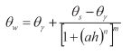
The provided permeability functions and coefficients are listed below.

• Gardner coefficient

 : Permeability ratio (permeability coefficient according to h increase / permeability coefficient at h=0)

a, n : Experimental constants predicted from Curve Fitting of unsaturated experimental data

• Frontal function

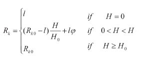
K ratio (Rk) : Permeability ratio (permeability coefficient according to h increase / permeability coefficient at h=0)

Ho : Head at which the permeability coefficient no longer decreases

• Van Genuchten function (Permeability ratio)

: Permeability ratio (permeability coefficient according to h increase / permeability coefficient at h=0)

a, n, m : Experimental constants predicted from Curve Fitting of unsaturated experimental data

• Van Genuchten (Water content)

: Volume water content

: Residual volume water content

: Saturated volume water content

a, n, m : Experimental constants predicted from Curve Fitting of unsaturated experimental data

[Relation]

The unsaturated material property data can be set on the ground type according to the JICE (Japan Institute of Construction Eng.) criteria. The pressure head-volumetric water content (degree of saturation)-permeability ratio relationship function for each type of ground is shown below.

<Dual consideration>

For unsteady analysis, the negative pressure head (pore water pressure) is calculated for each time step (construction step) and applied, renewing the relative permeability coefficient. The volumetric water content (degree of saturation), according to the calculated pressure head, is found and the relative permeability, according to the found volumetric water content (degree of saturation), is renewed for each step.

Strain compatible function

For the 2D equivalent linear analysis, the shear modulus and damping ratio are set as functions of strain to consider the nonlinearity and inelastic behavior of the ground. If the function is not defined, the ground material is assumed to be linear and the entered (fixed) shear modulus and damping ratio is applied. Generally, the ground displays decreasing shear modulus and increasing damping ratio as the shear strain increases. For complex nonlinear behavior of the ground, the material properties are simplified to linear equivalent properties. Repeated calculations from the assumed initial values can compute the converging shear modulus and damping ratio.

Material properties can be defined from various existing database. The following empirical equation can be used to generate a function following the stratum properties.

[Database]

A strain function stored from existing research can be imported from the database. An example DB is shown below.

Response spectrum function

Define the spectrum function used in response spectrum analysis. Because the response spectrum analysis uses a linearly interpolated spectrum function value for the natural periodicity of the structure, compact spectrum values are needed for areas where the curvature of the spectrum curve changes rapidly. The period range of the spectrum function must contain all natural periods of the structure.  

The spectrum data types are normalized acceleration (acceleration spectrum, gravitational acceleration), acceleration, velocity and displacement spectrum and changing the time function data format only changes the application format, not the data format. The scale factor is a gradient modulus for the entered data and the entire data can be scaled to fit the specified maximum value. In the 'Damping Ratio' space, input the damping ratio applied on the response spectrum but if the damping ratio of the target structure is different, the input spectrum data is processed to fit the structural damping ratio.

[Design spectrum function]

Use the built-in design spectrum. The default built-in design spectrum types are as follows.

• Korea(Bridge) : Korea, Traffic Specification

• Japan(Bridge02) : Japan, Load instruction and Dynamic Analysis of Building

• China(JTJ004-89) : China, Specifications of Earthquake Resistant Design for Highway Engineering

• KBC 2009 : Korea, Korea Building Code-Structural 2009

• KBC 2005 : Korea, Korea Building Code-Structural 2005

• IBC2000(ASCE7-98) : USA, International Building Code 2000

• UBC(1997) : USA, Measure of Uniform Building Code 97 (Standards)

• EURO(2004H-ELASTIC) : Europe, Sesismic Design Measure of Structures

Time forcing function

The time forcing function is applied to the loading conditions (ground acceleration, time varying static, dynamic nodal, dynamic surface) applied to linear/nonlinear time history analysis. A function for the time history loading value is formed and changing the time function data format only changes the application format, not the data format.[edit] The scale factor is a gradient modulus for the entered data and the entire data can be scaled to fit the specified maximum value.

[Add Time Function]

The defined function is also applicable for Dynamic node (surface) loading and time varying static loading. Specifying 'Force' or 'Moment' uses the time history load as a 'dynamic node (surface) load' input and specifying 'Normalized Acceleration' or 'Acceleration' uses it to input the 'ground acceleration'. Specifying 'Normal' uses the time history load as the change in static load with time for 'time varying static load' or 'dynamic surface load'.

[Import/Earthquake]

Save and import frequently used time history loading or select earthquake acceleration data from the program DB. There are a total of 32 types of earthquake acceleration.

[Add Time Sinusoidal]

A sine function can be used to define the time history loading. A, C are constants, f is the frequency of the input load, D is the damping factor and P is the phase angle. If the time history load is entered as a harmonic function, input the necessary sine function variables and click [Redraw Graph] to view the loading on the right hand side.