Solid Stresses
| ||||||||||||||||||||||||||||||||||||||||||||
|
| ||||||||||||||||||||||||||||||||||||||||||||
|
| ||||||||||||||||||||||||||||||||||||||||||||
|
Check the stress distribution of solid elements in Contours.
Analysis results (stresses) for Moving Load Analysis can be now produced. | ||||||||||||||||||||||||||||||||||||||||||||
|
| ||||||||||||||||||||||||||||||||||||||||||||
|
| ||||||||||||||||||||||||||||||||||||||||||||
|
| ||||||||||||||||||||||||||||||||||||||||||||
|
From the Main Menu select Results > Stresses > Solid Stresses.
Select Results > Stresses > Solid Stresses in the Menu tab of the Tree Menu.
Click | ||||||||||||||||||||||||||||||||||||||||||||
|
| ||||||||||||||||||||||||||||||||||||||||||||
|
| ||||||||||||||||||||||||||||||||||||||||||||
|
|
 Solid Stresses
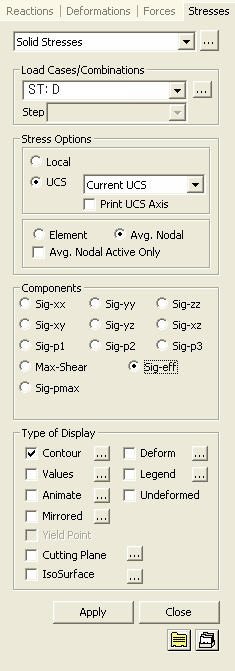
|
Contour |
Display the stresses of solid elements in contour. |
|
|
Ranges: Define the contour ranges.
Note
Number of
Colors: Assign the number of colors to be included in the contour
(select among 6, 12, 18, 24 colors) Colors: Assign or control the colors of the contour.
Color Table: Assign the type of Colors.
Reverse Contour: Check on to reverse the sequence of color variation in the contour.
Contour Line: Assign the boundary line color of the contour
Element
Edge: Assign the color of element edges while displaying the contour Contour Options: Specify options for contour representation
Contour Fill
Gradient
Fill: Display color gradient (shading) in the contour.
Draw Contour
Line Only
Mono line: Display the boundaries of the contour in a mono color.
Contour
Annotation
Spacing: Specify the spacing of the legend or annotation.
Coarse Contour
(faster) (for large plate or solid
model)
Extrude The option is not concurrently applicable with the Deformed Shape option. Similarly, the option cannot be concurrently applied to the cases where the Hidden option is used to display plate element thicknesses or the Both option is used to represent Top & Bottom member forces (stresses). |
 : Assign the color distribution
range of contour. Using the function, specific colors for specific ranges
can be assigned.
: Assign the color distribution
range of contour. Using the function, specific colors for specific ranges
can be assigned. : Control the colors by zones
in the contour.
: Control the colors by zones
in the contour.|
Deform |
Display the deformed shape of the model. |
|
|
Deformation
Scale Factor Deformation
Type
Nodal Deform: Display the deformed shape only with nodal displacements.
Real Displacement
(Auto-Scale off): The true deformation
of the structure is graphically represented without magnifying or reducing
it. This option is typically used for geometric nonlinear analysis reflecting
large displacement. Relative Displacement: The deformation of the structure is graphically represented relative to the minimum nodal displacement, which is set to "0" |
|
Values |
Display the stresses of solid elements in numerical values. The font and color of the numbers can be
controlled in |
|
|
Decimal
Points: Assign decimal points for the displayed numbers. Min &
Max: Display the maximum and minimum values. Set Orientation: Display orientation of numerical values.
Note |

|
Legend |
Display various references related to analysis results to the right or left of the working window. |
|
|
Legend Position: Position of the legend in the display window
Rank Value Type: Specify a type of values in the Legend and the number of decimal points. |
|
Animate |
Dynamically simulate the stresses of the solid elements. Click |
|
|
Animation Mode: Determine the type of animation for analysis results.
Animate
Contour: Option to change the color of the contour representing
the transition according to the magnitudes of variation
Note AVI Options: Enter the options required to produce the animation window.
Bits per
Pixel: Number of bits per pixel to create the default window for
animation Construction Stage Option: Select the animation options when the construction stage analysis is performed.
Stage Animation:
Animations by construction stages |
 then click
  Record to the right of the Animation control board at the
bottom of the working window.
Record to the right of the Animation control board at the
bottom of the working window. : Assign the method of compressing image data
|
Undeformed |
Overlap the undeformed and deformed shapes of the model. |
|
Mirrored |
"Mirrored" allows the user to expand the analysis results obtained from a half or quarter model into the results for the full model by reflecting planes. |
|
|
Half Model Mirroring |
|
Yield Point |
If the analysis results produced by material nonlinear analysis exceed the yield stress of Plastic Material defined in Initial Uniaxial Yield Stress, Hinge is produced at Gauss Point. |
[Check the results obtained from the analysis of masonry materials]
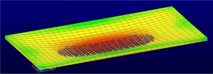
Figure 1. Principle stresses and crack positions ?under gravity loads
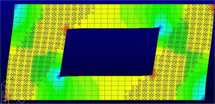
Figure 2. Principle stresses and cracks positions - under lateral loads
|
Cutting Plane |
Graphically display the stresses of the solid elements along a cutting plane. |
|
|
Click |
|
|
Named Planes
for Cutting
Outline
Type
Free Face:
Draw the outline of all the faces that are not in contact with other solid
elements.
Animation
Option
Global X
Sweep: Produce a stress contour animation for the cut plane by
moving the cutting plane toward GCS X-direction |
.jpg)
 : Detailed display options
for animation.
: Detailed display options
for animation.|
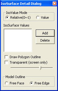
IsoSurface |
IsoSurface searches and displays the planes of equal stresses resulting from Heat of Hydration analysis within the solid elements. |
|
|
IsoValue
Mode Relative(0~1) IsoSurface
Values
Draw
Polygon Outline Model Outline
Free Face:
Draw the outline of all the faces that are not in contact with other solid
elements. Note |
 button to enter a numerical value. Multiple entries
are possible.
button to enter a numerical value. Multiple entries
are possible. : Click the button to delete data entries.
 Batch Output Generation (
  ,
,  )
)
Given the types of analysis results for Graphic outputs, generate consecutively graphic outputs for selected load cases and combinations. A total number of files equal to the products of the numbers of checked items in the three columns of the dialog box below are created.
|
|
Assign a Base File Name under which the types of results (selection data in the Batch Output Generation dialog box for graphic outputs) are stored. |
|
|
Specify the Base Files to perform Batch Output Generation, construction stages, load cases (combinations), steps, etc. in the following dialog box. |
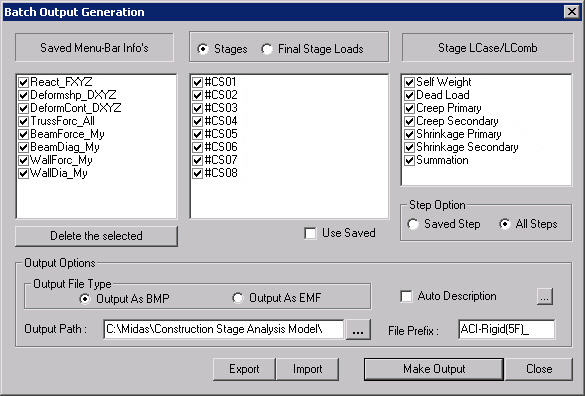
Batch Output Generation dialog box
Saved Menu-Bar Info's: Listed here are the Base Files. Select the Base File Names for Batch Output.
 : Delete all the Base Files selected with the mouse.
When the construction stage analysis is carried out, all the construction stages are listed. We simply select the stages of interests to be included in the batch output. If no construction stage analysis is performed, the column in the dialog box becomes inactive and lists load (combination) conditions.
Stages
The results output of all the construction stages are produced. The construction
stages are listed below.
Final Stage
Loads
The results output for only the Final Stage are produced. The construction
stages are listed below. If no construction stage analysis is performed,
the load (combination) conditions are listed.
Use Saved
Apply only the (saved) step or load (combination) condition selected at
the time of creating each Base File.
Stage LCase/LComb
When the construction stage analysis is carried out, the auto-generated
construction stage load conditions and the additionally entered construction
stage load combinations are listed. Check on only the load (combination)
conditions that will be used to produce batch outputs. This column becomes
inactive if Final Stage Loads?is selected or no construction stage analysis
is carried out.
Step Option
Specify the steps for which the outputs will be produced when the construction
stage analysis or large displacement geometric nonlinear analysis is performed.
Saved Step: Use only the steps used for creating the Base Files
All Steps: Use all the steps
Output Options
Output
File Type
Select a Graphic File type, either BMP or EMF.
Auto Description:
At the top left of the Graphic Outputs produced in batch, auto-generate
and include the notes such as the types and components of the analysis
results, construction stages and steps, load (combination) conditions,
etc. The font size, color, type, etc. can be changed upon clicking the
button  .
.
Output
Path
Specify the path for saving the graphic files to be produced in batch.
File Prefix: Specify the prefix of the Graphic Files to be created. The filenames will be consisted of "Prefix"_"Base File Name"_"Load Comb.".bmp(emf) or "Prefix"_"Base File Name"_"Stage"_"Stage LCase"_"Step".bmp(emf).
 : Produce the specified batch
Graphic Files reflecting the contents of the dialog box.
: Produce the specified batch
Graphic Files reflecting the contents of the dialog box.
 /
/ 
Produce the contents of data input in the
Base Files and Batch Output Generation dialog box in a binary type file
(fn.bog). Click the button and select a fn.bog to use
the same output format.
Note
Import /Export is only meaningful for different projects. In a given structural
model, the Base Files are automatically stored and listed.