Example:  Slope Stability Analysis based on Stress Analysis Method

The limit equilibrium method based on the simplified Bishop formulation is a popular approach to the 2D slope stability problem due to its simplicity and convenience. In commonly available software, this approach is combined with the method of slices to determine the static equilibrium. The method of slices, however, is based on several simplified assumptions. For instance, it usually cannot take into account the effects of ground water changes or of construction stages (stress path history in plastic materials). The use of finite element analysis to determine static equilibrium can overcome these limitations.

In GTS, a new type of 2D analysis is therefore made available: Slope Stability based on Stress Analysis Method (SAM). In this approach, the limit equilibrium method is applied to a state of stress in static equilibrium computed using non-linear finite element analysis. After the user specified a family of slip surfaces to be checked, the analysis determines the factor of safety and the critical slip surface.

This new analysis type is complementary to the existing Slope Stability (SRM) analysis based on the Strength Reduction Method.

Slope Stability based on Stress Analysis Method consists of 5 steps:

Step 1 : The user creates a model of the slope

(define the geometry of the model, soil property, boundary and load)

Step 2 : The user defines a suitable family of slip surfaces

Step 3 : The user selects the analysis type ‘Slope Stability (SAM)’ and runs the FEM analysis

Step 4 : GTS smoothes the resulting stress field

Step 5 : GTS calculates the safety factor for each slip surface and identifies the critical case.

[Step 1] Modeling of the Slope

Slope Stability (SAM) is restricted to 2D analysis. Nevertheless, all element types, all material models, all loads and all boundary conditions available in 2D non-linear analysis can be used in Slope Stability (SAM).

The user should specify ground densities in the material dialog and apply the gravity load.

[Step 2] Define families of slip surfaces

The user needs to specify the general shape and the positioning of a family of slip surfaces that will be checked for stability. In midas GTS, these can be specified using the menu ‘Model > Boundary > Slip Surface (Circular)’ or 'Model > Boundary > Slip Surface (Polygonal).'

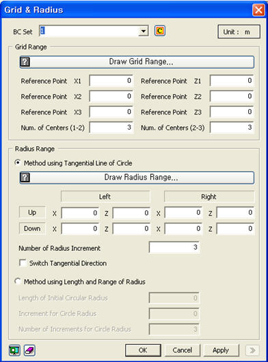
Figure 1: Dialog Box for a Circular Surface

The circular surface function defines a family of slip surfaces in terms of centers and radii. First, the family of centers can be specified using the Grid Range input, see figure 1.

The Grid Range input specifies a non-orthogonal grid of center points, as shown in figure 2.

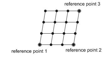
Figure 2: Reference Points of Grid Range

In the input dialog, x1 and z1 correspond to the coordinates of ‘Reference Point 1’. Similarly, x2, z2 and x3, z3 refer to the coordinates of ‘Reference Point 2’ and ‘Reference Point 3,’ respectively. These points can be created by mouse-clicking or by entering the coordinates manually.

Num. of Centers (1-2) defines the number of divisions between Reference Points 1 and 2. Num. of Centers (2-3) defines the number of divisions between Reference Points 2 and 3.

An example with Num. of Centers (1-2) = 5 and with Num. of Centers (2-3) = 3 is shown in Figure 3.

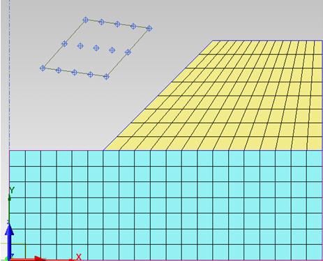
Figure 3: Example of Grid Range Input

Two methods are available for defining the radii. One is the Method using the Tangential Line of a Circle, and the other one is the Method using the Length and Range of the Radius.

Method using the Tangential Line of a Circle

This method allows the definition of two extreme tangent lines by inputting the coordinates of four points (mouse clicking or manual input), as shown in figure 4. The ‘number of radius increments’ defines the number of straight lines that will be additionally created by dividing the distance between the upper straight line and the lower straight line. Figure 4 shows the case where the number of radius increments is 4.

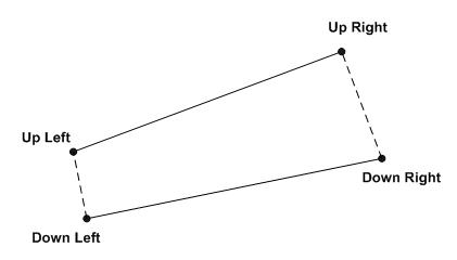
Figure 4: Input Point for the Method using Tangential Line

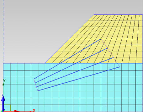
Figure 5: Input Examples for the Method using the Tangential Line

The length of each radius can be calculated as the shortest distance between the considered center point (from the grid range) and the considered tangent line. For instance, if the total number of center points is 12, and the number of tangent lines is 4, the total number of trial Slip Surfaces is 48 (12 x 4).

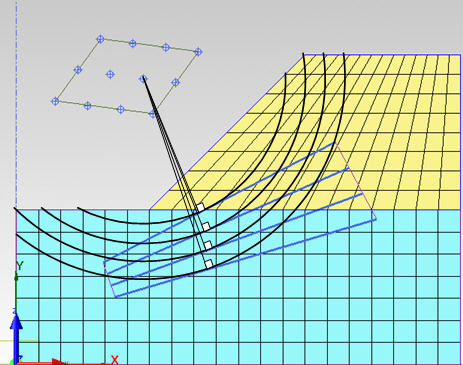
Figure 6: Trial Slip Surfaces using the Tangential Line of a Circle

Method using the Length and Range of the Radius

The method using the radius requires three input items: Length of Initial Radius, Length of Increments, and Number of Increments. A warning message will appear if one of the defined circles does not intersect with the model.

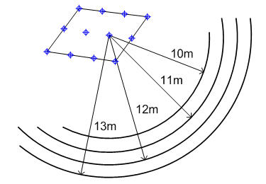
Figure 7: Example of Method using the Radius

Polygonal Surface

The Polygonal Surface function is an alternative option to define the shape of slip surfaces. Each polygonal line can be defined either using mouse clicks or manually entering coordinates.

In the case where coordinates are defined through mouse clicking, the selected points can be checked in a table, as shown in figure 10.

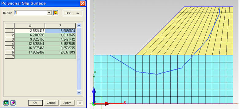
Figure 10: Input Examples of Polygonal Surfaces

[Step 3] Perform slope stability analysis (SAM)

In order to compute the static equilibrium of stress field, an analysis case of type ‘Slope Stability (SAM)’ must be created and run. Note that the ground water level can be defined as an equation or as a multi-linear diagram in the Analysis Control dialog box.

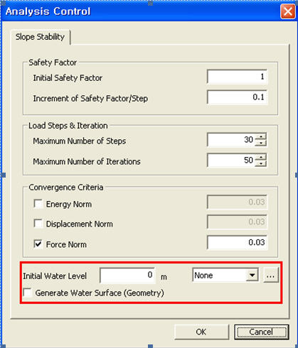
Figure 11: Input Dialog for Ground Water Level during Slope Stability Analysis

[Step 4] Smoothing of the resulting stress field

The integration of stresses along trial slip surfaces requires Co continuity of the stress field. Since the resultant stress field from finite element methods could be discontinuous at element boundary, it is necessary to smooth the FEM stress results to obtain a continuous stress field over the whole model before integration. The stress smoothing method proposed by Hinton and Campbell (1974) is adopted.  In this method, the shape functions, N, which is generally used for the interpolation of displacements from nodal values, is adopted as piecewise interpolation functions to obtain the continuous stress field. The degrees of freedom of this interpolation are unknown stress values at the nodes of the finite element mesh. Unknown nodal stress values are determined by minimizing of the distance between the discontinuous FEM stress field and the continuous interpolated stress field.

 [Step 5] Calculate the Factor of Safety

• The factor of safety used in the Stress Analysis Method is computed by integration over the slip surface.

• Numerical integration of the smoothed stress field along the Slip Surface.

• The stress integration along the slip surface in the global coordinate system is calculated.

• Determination of the factor of safety of the slope

• The factor of safety is computed for all trial slip surfaces specified by the user. The slip surface with the lowest factor of safety is identified as the critical slip surface. The lowest value is identified as the factor of safety of the slope.